Non-perturbative spectral gravity measure
in the Hilbert–Schmidt Gaussian completion:
pro-torsor structure and the obstruction
to canonical expectations

David Alfyorov, Igor Shnyukov
Independent researchers
davidich.alfyorov@gmail.com

Abstract

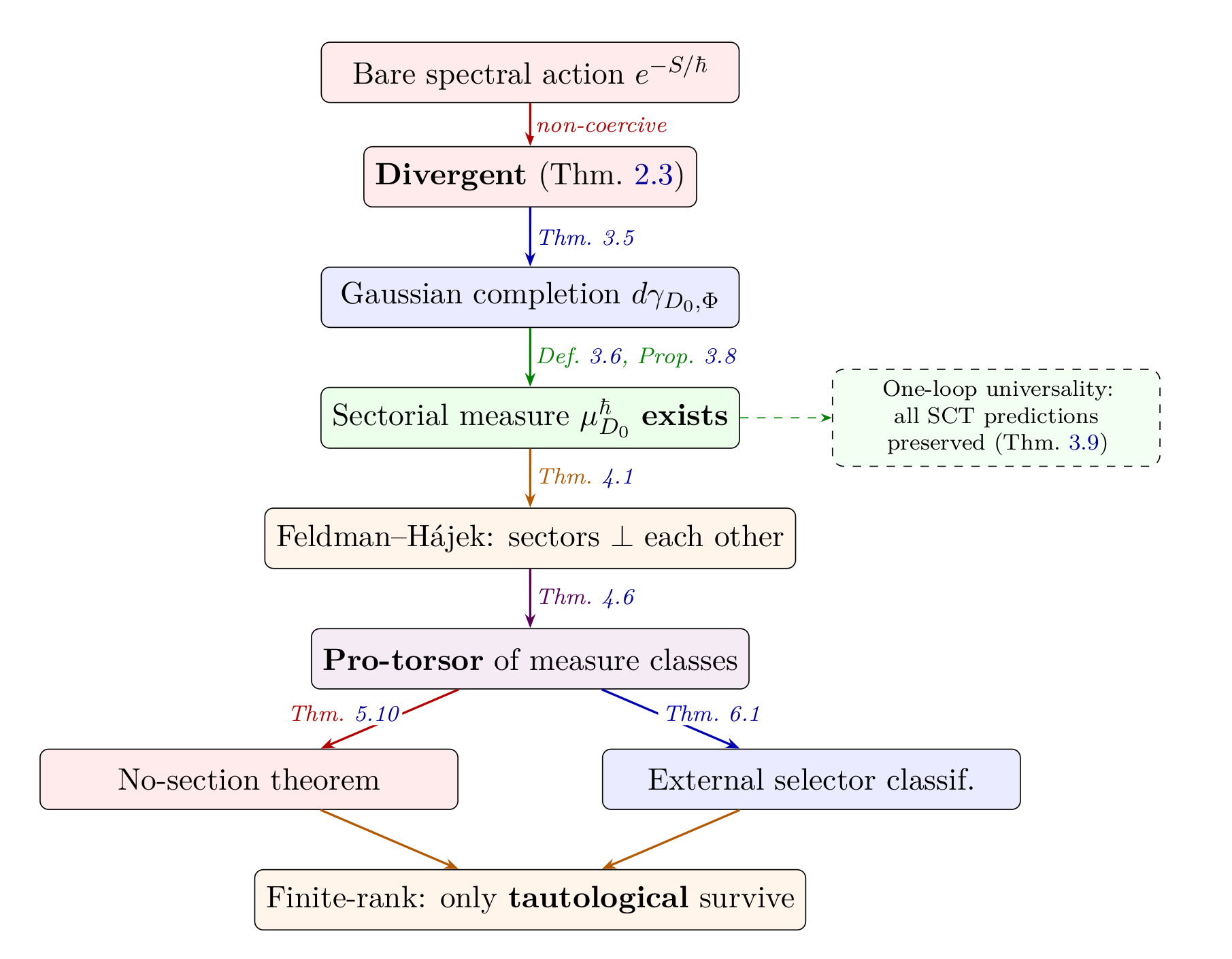
We construct rigorous non-perturbative sectorial measures for the spectral action on Dirac operators with compact resolvent within the Hilbert–Schmidt Gaussian completion framework and classify the global obstruction to assembling them into a single functional integral. The naive Euclidean weight $\exp(-\operatorname{Tr}f(D^{2}/\Lambda^{2}))$ is non-coercive and yields a divergent integral; we cure this by introducing a two-sided functional Gaussian reference measure on the Hilbert–Schmidt self-adjoint fluctuation space $\mathrm{HS}_{\mathrm{sa}}(H)$ , with covariance determined by the background spectral data. The completed sectorial measure exists, has finite partition function, and is projectively compatible across spectral truncation ranks. Different background sectors, however, produce mutually singular Gaussian classes (Feldman–Hájek rigidity), preventing the assembly of a single background-independent probability measure within this framework. The resulting global object is a pro-torsor of local completed measure classes equipped with a dual density-valued observable sheaf. We prove a principal no-section theorem: relative to any choice of reference weight $\Phi$ , the bounded density gauge group acts freely on normalized projective representatives, precluding further canonical reduction to a scalar-probability trivialization without additional structure. External scalar completion is classified exactly: it requires sector weights and sectorial terminal densities, subject to a truncation-sufficiency criterion. At finite spectral rank, every separating state-independent selector channel must be injective, hence a tautological re-encoding of the full truncation; under a non-tautology axiom this yields a complete no-go. The one-loop predictions reported in the companion SCT papers are shown to be universally preserved, independent of the choice of Gaussian reference, within the present framework.

Keywords: spectral action, non-perturbative measure, pro-torsor, Feldman–Hájek singularity, density-valued observables, noncommutative geometry

MSC 2020: 81T16, 58J42, 46L87, 28C20, 81T13

1 Introduction

The spectral action principle, introduced by Chamseddine and Connes [15, 16], postulates that the bosonic dynamics of gravity coupled to matter is governed by the functional

	$S[D]\;=\;\operatorname{Tr}\,f\!\left(\frac{D^{2}}{\Lambda^{2}}\right),$		(1)

where $D$ is the Dirac operator of an almost-commutative spectral triple encoding the Standard Model coupled to Euclidean gravity, $\Lambda$ is a high-energy cutoff scale, and $f\colon[0,\infty)\to[0,\infty)$ is a positive even Schwartz-class test function. The classical content of this action–the Einstein–Hilbert term, cosmological constant, Higgs potential, and gauge kinetic terms–is recovered from the asymptotic expansion of (1) in powers of $\Lambda^{-2}$ [16, 14, 28].

While the classical spectral action has been extensively studied, the quantum theory–the functional integral over Dirac operators,

	$Z\;=\;\int\exp\!\bigl(-S[D]/\hbar\bigr)\,\mathcal{D}[D],$		(2)

–remains largely formal. At finite spectral rank, Barrett and Glaser [12] computed the integral over random noncommutative geometries via Monte Carlo methods, and subsequent work by Azarfar–Khalkhali [11] and Perez-Sanchez [25] studied the functional renormalization group for matrix-model truncations. At one loop, van Nuland and van Suijlekom [27] gave a rigorous treatment of one-loop corrections to the spectral action. However, the full non-perturbative measure $\mathcal{D}[D]$ on the infinite-dimensional space of Dirac operators has not been constructed.

This paper addresses the non-perturbative measure problem directly. Our main results are:

1.

The naive integral (2) diverges: the bare Euclidean weight is bounded below by a positive constant and the configuration space is non-compact (Theorem 2.3).
2.

A corrected two-sided functional Gaussian reference measure on the self-adjoint Hilbert–Schmidt fluctuation space $\mathrm{HS}_{\mathrm{sa}}(H)$ yields a well-defined sectorial completed measure for each compact-resolvent background $D_{0}$ (Theorem 3.5, Definition 3.6, and Proposition 3.8).
3.

Different background sectors produce mutually singular Gaussian classes via Feldman–Hájek rigidity, even for perturbatively adjacent backgrounds (Theorem 4.1, Proposition 4.3). The global object is therefore a pro-torsor of local completed measure classes (Theorem 4.6).
4.

Chart-independent expectations of ordinary scalar observables are not canonically defined; only sections of a dual density line pair canonically with the pro-torsor (Theorem 4.8).
5.

No internal axiom (symmetry, semiclassical matching, background covariance, finite-observable data, or tail/asymptotic selection) can trivialize the pro-torsor: the bounded density gauge group acts freely on normalized representatives (principal no-section theorem, Theorem 5.10).
6.

External scalar completion is classified by sector weights and sectorial terminal densities satisfying a truncation-sufficiency criterion (Theorem 6.1). At finite spectral rank, every separating state-independent selector channel must be injective and hence a tautological re-encoding of the full truncation (Theorem 6.6).
7.

All tree-level and one-loop predictions of spectral causal theory are universally preserved, independent of the choice of Gaussian reference (Theorem 3.9).

Contribution. The present work provides the first rigorous construction of non-perturbative sectorial measures for the spectral action, together with a classification of the obstruction–within the Gaussian Hilbert–Schmidt framework–to assembling them into a single background-independent functional integral with ordinary scalar expectations. The positive content is that sectorial measures exist and are projectively compatible. The negative content is that no internal principle can assemble them into a single background-independent probability measure; the missing data is external and precisely classified. This parallels the well-known necessity of boundary data in canonical quantum gravity [26, 7] and holographic settings, but here the necessity emerges as a mathematical theorem within the spectral action framework rather than being imposed as an external assumption.

Status. The pro-torsor construction and the principal no-section theorem are proven unconditionally. The external classification and finite-rank tautology theorem are proven. The full no-go (no admissible non-tautological selector tower) is conditional on an explicit non-tautology axiom. Lorentzian continuation and the interface with the fakeon prescription [9] are not addressed; see Section 9.

The paper is organized as follows. Section 2 recalls the spectral action and proves divergence of the naive integral. Section 3 introduces the corrected Gaussian reference and establishes sectorial existence. Section 4 constructs the pro-torsor and proves the scalar-expectation no-go. Section 5 proves all internal no-go theorems, culminating in the principal no-section theorem. Section 6 classifies external selectors and proves the finite-rank tautology theorem. Section 7 sketches the application to the Standard Model spectral triple. Section 8 compares with other approaches to quantum gravity. Section 9 states what the paper does not show and gives the conclusion.

Figure 1: Logical structure of the paper. The bare spectral action weight is non-coercive and yields a divergent integral. A Gaussian reference cures this sectorially, but the Feldman–Hájek singularity between sectors forces a pro-torsor structure. No internal axiom can trivialize the torsor (principal no-section theorem); external data is classified but constrained to tautological finite-rank channels. All one-loop predictions are universally preserved.

2 The spectral action and its measure problem

2.1 Setup

Let $(H,D_{0},\gamma,J)$ be a compact-resolvent even real spectral triple, where $H$ is a separable Hilbert space, $D_{0}$ is a self-adjoint operator with compact resolvent $D_{0}e_{n}=\lambda_{n}e_{n}$ , $\gamma$ is the grading, and $J$ is the real structure. We denote the eigenvalues in non-decreasing order of $|{\lambda_{n}}|$ .

The self-adjoint Hilbert–Schmidt fluctuation space is

	$X\;:=\;\mathrm{HS}_{\mathrm{sa}}(H)\;=\;\bigl\{A\in B(H):A=A^{*},\;\operatorname{Tr}(A^{2})<\infty\bigr\},$		(3)

equipped with the Hilbert–Schmidt inner product $\langle A,B\rangle_{\mathrm{HS}}=\operatorname{Tr}(AB)$ .

Remark 2.1 (Choice of configuration space and gauge fixing).

In the noncommutative-geometry framework, the physical inner fluctuations $A=\sum a_{i}[D,b_{i}]$ are bounded operators but not necessarily Hilbert–Schmidt. We work on $\mathrm{HS}_{\mathrm{sa}}(H)$ because it is the largest space on which centered Gaussian probability measures with trace-class covariance exist (see Section 3). The divergence argument of Theorem 2.3 applies a fortiori on any subspace of $\mathrm{HS}_{\mathrm{sa}}(H)$ , and extends to any ambient space admitting a reference measure, since the spectral action remains bounded by $(\dim H)\,f(0)$ on $\mathrm{HS}_{\mathrm{sa}}(H)$ and converges to a finite limit along every ray. On spaces of unbounded operators where the spectral action may become coercive, the measure problem takes a different form; this is beyond our scope. We emphasize that inner fluctuations of almost-commutative spectral triples (gauge connections, Higgs fields) are bounded operators that are not Hilbert–Schmidt in general: a smooth multiplication operator on a compact manifold is bounded but not compact. The restriction to $\mathrm{HS}_{\mathrm{sa}}(H)$ is therefore a genuine mathematical choice, not a physical requirement. Its justification is that the Gaussian reference (Theorem 3.5) requires trace-class covariance, which exists only on $\mathrm{HS}_{\mathrm{sa}}(H)$ or its subspaces. What is excluded are large fluctuations far from any background–precisely the configurations where the one-loop approximation breaks down. The non-perturbative measure problem for such configurations requires different tools (e.g., lattice or CDT-type discretization [7]) and lies beyond the scope of this work.

An important open question is whether the pro-torsor obstruction (Section 4) persists on a larger configuration space. On a space where the spectral action is coercive, the Gaussian reference may be unnecessary, and the Feldman–Hájek singularity–which is driven by the product structure of the Gaussian covariance–may not arise. Conversely, non-Gaussian references (e.g., Radon measures on spaces of bounded operators) could generate a different obstruction landscape. Until this question is settled, the results of this paper should be understood as applying to the Gaussian-completed Hilbert–Schmidt framework, not as unconditional statements about the spectral action in general. Furthermore, the spectral action is invariant under unitary conjugation $D\to UDU^{*}$ ; the construction in this paper is performed on a fixed background sector where the gauge is implicitly fixed by the choice of $D_{0}$ . The Feldman–Hájek singularity of Theorem 4.1 concerns the Gaussian classes attached to different Hilbert–Schmidt background charts $\mathcal{C}(D_{0})=D_{0}+\mathrm{HS}_{\mathrm{sa}}(H)$ . If $D_{0}^{\prime}=UD_{0}U^{*}$ is gauge-equivalent to $D_{0}$ , the natural comparison is the chart-to-chart isomorphism $J_{U}(A)=UAU^{*}$ , which is an isometry on $X$ satisfying $(J_{U})_{*}\gamma_{D_{0},\Phi}=\gamma_{D_{0}^{\prime},\Phi}$ and $(J_{U})_{*}\mu^{\hbar}_{D_{0}}=\mu^{\hbar}_{D_{0}^{\prime}}$ (because $C_{D_{0}^{\prime},\Phi}(J_{U}A)=J_{U}(C_{D_{0},\Phi}(A))$ and $S_{D_{0}^{\prime}}(J_{U}A)=S_{D_{0}}(A)$ by trace invariance). Thus gauge-equivalent backgrounds do not generate a new Feldman–Hájek singularity; they give isomorphic measured sectors. The affine formula $A\mapsto UAU^{*}+U[D_{0},U^{*}]$ arises only when the transformed sector is re-expressed back in the original chart; for almost-commutative Standard Model backgrounds the pure-gauge term $U[D_{0},U^{*}]$ is generically a bounded multiplication operator but not Hilbert–Schmidt (a non-zero smooth multiplication operator on a compact manifold is bounded but not compact), so this fixed-chart re-expression is not an action on $X$ . The Cameron–Martin obstruction of Appendix B applies to such fixed-chart translations (geometric chart shifts, which correspond to diffeomorphisms—an outer symmetry distinct from the inner gauge group in NCG), not to the chart-to-chart identification $J_{U}$ . Accordingly, Theorem 4.1 should be interpreted as an obstruction between gauge-inequivalent background sectors (distinct spectra = distinct gauge orbits), while a fully global quotient-level construction still requires an explicit gauge-fixed atlas and Faddeev–Popov analysis; see Section 9.

For a fixed background $D_{0}$ , the total Dirac operator is $D=D_{0}+A$ with $A\in X$ . The spectral action evaluated on the fluctuation is

	$S(A)\;:=\;\operatorname{Tr}\,f\!\left(\frac{(D_{0}+A)^{2}}{\Lambda^{2}}\right),$		(4)

where $f\colon[0,\infty)\to[0,\infty)$ is a positive even Schwartz-class function.

2.2 Divergence of the naive integral

The positivity and boundedness of $f$ immediately constrain $S$ :

Lemma 2.2.

For every $A\in X$ , $S(A)\geq 0$ . On any finite-rank slice $\Omega_{N}$ of dimension $d_{N}$ ,

	$0\;\leq\;S_{N}(A)\;\leq\;d_{N}\,f(0).$		(5)

In infinite dimensions ( $\dim H=\infty$ ), the full spectral action $S(A)=\sum_{j}f(\mu_{j}^{2}/\Lambda^{2})$ is finite for every $A$ (since $f$ is Schwartz and $D_{0}+A$ has Weyl-growing eigenvalues), but $S(A)\leq S(0):=\sum_{j}f(\lambda_{j}^{2}/\Lambda^{2})<\infty$ does not hold in general.

Proof.

Since $f\geq 0$ , every summand $f(\mu_{j}^{2}/\Lambda^{2})\geq 0$ , giving $S\geq 0$ . On $\Omega_{N}$ , there are $d_{N}$ eigenvalues, each contributing at most $f(0)$ . ∎

Theorem 2.3 (Divergence of the naive integral).

Let $V\subset X$ be any nonzero finite-dimensional subspace. Then

	$\int_{V}\exp\!\bigl(-S(A)/\hbar\bigr)\,\mathrm{d}A\;=\;+\infty.$		(6)

Proof.

It suffices to show that $\exp(-S(A)/\hbar)$ is bounded below by a positive constant along every ray in $V$ , since $V$ contains unbounded rays and the resulting lower-bounded integral over each ray diverges.

Fix any nonzero $A_{1}\in V$ and consider the ray $A(t)=tA_{1}$ , $t\in\mathbb{R}$ . The operator $D(t):=D_{0}+tA_{1}$ has eigenvalues $\mu_{n}(t)$ . Since $A_{1}\in\mathrm{HS}_{\mathrm{sa}}(H)$ is compact, Weyl’s inequality gives $|\mu_{n}(t)-\lambda_{n}|\leq t\,\|A_{1}\|$ , so $|\mu_{n}(t)|\geq|\lambda_{n}|-|t|\,\|A_{1}\|$ . For each fixed $t$ , the spectral tail satisfies $|\mu_{n}(t)|\to\infty$ as $n\to\infty$ , hence $f(\mu_{n}(t)^{2}/\Lambda^{2})\to 0$ along the tail (since $f\geq 0$ and $f(u)\to 0$ as $u\to\infty$ ).

The action $S(tA_{1})=\sum_{n}f(\mu_{n}(t)^{2}/\Lambda^{2})$ is therefore a convergent sum of non-negative terms, each bounded by $f(0)$ . As $|t|\to\infty$ , the eigenvalues of $D(t)$ are pushed away from the origin: for any fixed $R>0$ , only finitely many indices $n$ satisfy $|\mu_{n}(t)|\leq R$ when $|t|$ is large (since $|\lambda_{n}|$ grows and $A_{1}$ is compact). Therefore the number of terms contributing more than $\delta$ to the sum tends to zero, and $S(tA_{1})\to c_{A_{1}}$ for some finite $c_{A_{1}}\geq 0$ .

Hence $\exp(-S(tA_{1})/\hbar)\to\exp(-c_{A_{1}}/\hbar)>0$ , and the integral along the ray $\int_{-\infty}^{\infty}\exp(-S(tA_{1})/\hbar)\,\mathrm{d}t=+\infty$ (by comparison with a positive constant on an unbounded interval). Since $V$ contains such a ray, the $d$ -dimensional integral over $V$ diverges. ∎

Remark 2.4.

Theorem 2.3 shows that neither a global minimum principle nor a naive path integral is available for the spectral action. The weight $\exp(-S/\hbar)$ is essentially constant at infinity, and the configuration space is non-compact. A completion of the exponent–by a reference measure, a coercive term, or a domain restriction–is mandatory.

2.3 Smooth-window truncations and convergence

For a smooth compactly supported cutoff $\chi_{R}\in C_{c}^{\infty}(\mathbb{R})$ with $0\leq\chi_{R}\leq 1$ , $\chi_{R}(\lambda)=1$ for $|\lambda|\leq R$ , and $\mathrm{supp}\,\chi_{R}\subset\{|\lambda|\leq R+1\}$ , define the smooth-window truncated action

	$S_{R}(A)\;:=\;\operatorname{Tr}\bigl(\chi_{R}(D_{0}+A)\,f((D_{0}+A)^{2}/\Lambda^{2})\bigr).$		(7)

Since $\chi_{R}(D_{0}+A)$ is a spectral function of $D_{0}+A$ , it commutes with all bounded Borel functions of $D_{0}+A$ , eliminating the projection/compression mismatch that afflicts frozen-projector truncations.

Theorem 2.5 (Smooth-window convergence).

Assume the following standard spectral-perturbation hypotheses:

(A1)

All operators $D(A):=D_{0}+A$ share a common dense domain $\mathrm{Dom}(D_{0})\subset H$ .
(A2)

The parameter derivatives $\partial_{i}D$ and $\partial_{ij}D$ are first-order differential operators with uniformly bounded matrix elements: $|\langle e_{m},\partial_{i}D\,e_{n}\rangle|\leq C(1+|\lambda_{m}|)^{1/2}(1+|\lambda_{n}|)^{1/2}$ .
(A3)

Uniform Weyl counting: $N_{A}(L):=\#\{n:|\mu_{n}(A)|\leq L\}\leq C_{K}(1+L)^{d}$ on compact parameter subsets $K$ .
(A4)

Schwartz divided differences: the first and second divided differences of any Schwartz function are again Schwartz on $\mathbb{R}^{2}$ and $\mathbb{R}^{3}$ , respectively.

Then for every compact parameter subset $K$ ,

	$\sup_{A\in K}\,\bigl\|\partial_{A}^{\alpha}\bigl(S_{R}(A)-S(A)\bigr)\bigr\|\;\longrightarrow\;0\qquad\text{as }R\to\infty,\quad\|\alpha\|\leq 2.$		(8)

If $f$ has Schwartz decay $|f^{(k)}(\lambda)|\leq C_{k}(1+|\lambda|)^{-M}$ for all $M$ , the convergence rate is

	$\bigl\|S_{R}(A)-S(A)\bigr\|\;\leq\;C_{K}\,(1+R)^{d-M}$		(9)

for any $M>0$ , with analogous estimates for derivatives. For exponentially decaying $f(\lambda)\sim e^{-c\lambda}$ , the rate is $\mathcal{O}(e^{-cR})$ .

Proof sketch.

Write $r_{R}:=(1-\chi_{R})\cdot h$ where $h(\lambda):=f(\lambda^{2}/\Lambda^{2})$ . Since $\chi_{R}=1$ for $|\lambda|\leq R$ and $h$ is Schwartz, $r_{R}\to 0$ in the Schwartz topology. The first derivative of the spectral action uses the Hellmann–Feynman formula (multiple operator integral of order 1), and the second derivative uses the double sum over divided differences. Under (A1)–(A4), the matrix element bounds and Weyl counting ensure uniform convergence of these sums. The rate estimate (9) follows from the tail bound $|r_{R}(\lambda)|\leq C(1+R)^{-M}$ for $|\lambda|>R$ . Full details are in Appendix A. ∎

Corollary 2.6 (Saddle persistence).

If $A_{*}=0$ is a nondegenerate critical point of $S$ on a gauge-fixed slice, then for all sufficiently large $R$ , $S_{R}$ has a unique nearby critical point $A_{R}\to A_{*}$ with converging Hessian.

3 Corrected functional Gaussian and sectorial existence

The divergence theorem motivates introducing an ambient reference measure that supplies the missing coercivity. We work with centered Gaussian measures on the operator space $X$ .

3.1 Two-sided functional Gaussian covariance

Definition 3.1.

Let $\Phi\colon[0,\infty)\to(0,\infty)$ be a positive admissible spectral weight (e.g., heat-kernel $\Phi(u)=e^{-u}$ or Sobolev $\Phi(u)=(1+u)^{-s}$ , $s>2$ ). Define the spectral decay coefficients $\phi_{n}:=\Phi(\lambda_{n}^{2}/\Lambda^{2})$ and the two-sided covariance operator

	$C_{\Phi}(A)\;:=\;\sigma^{2}\,\Phi_{0}\,A\,\Phi_{0},\qquad\Phi_{0}:=\Phi(D_{0}^{2}/\Lambda^{2}),$		(10)

acting on $X=\mathrm{HS}_{\mathrm{sa}}(H)$ , where $\sigma^{2}>0$ is a normalization constant.

In the eigenbasis $\{E_{mn}\}$ of $D_{0}$ , the covariance acts diagonally on matrix units: $C_{\Phi}(E_{mn})=\sigma^{2}\phi_{m}\phi_{n}\,E_{mn}$ .

Theorem 3.2 (Trace-class criterion).

The operator $C_{\Phi}$ is trace-class on $X=\mathrm{HS}_{\mathrm{sa}}(H)$ if and only if

	$\sum_{n=0}^{\infty}\phi_{n}\;<\;\infty.$		(11)

When this holds, $\operatorname{Tr}_{\mathrm{HS}}(C_{\Phi})=\sigma^{2}\bigl(\sum_{n}\phi_{n}\bigr)^{2}$ .

Proof.

Choose the real orthonormal basis of $\mathrm{HS}_{\mathrm{sa}}(H)$ consisting of the diagonal matrix units $F_{nn}:=E_{nn}$ and the off-diagonal units $(E_{mn}+E_{nm})/\sqrt{2}$ and $i(E_{mn}-E_{nm})/\sqrt{2}$ for $m<n$ . Then $C_{\Phi}(F_{nn})=\sigma^{2}\phi_{n}^{2}F_{nn}$ , contributing $\sigma^{2}\phi_{n}^{2}$ to the trace. Each off-diagonal pair contributes $\sigma^{2}\phi_{m}\phi_{n}$ . Summing: $\operatorname{Tr}_{\mathrm{HS}}(C_{\Phi})=\sigma^{2}[\sum_{n}\phi_{n}^{2}+2\sum_{m<n}\phi_{m}\phi_{n}]=\sigma^{2}(\sum_{n}\phi_{n})^{2}$ . This is finite iff $\sum_{n}\phi_{n}<\infty$ . ∎

Proposition 3.3 (Admissibility of standard spectral weights).

(a)

Heat-kernel: $\Phi(u)=e^{-\tau u}$ , $\tau>0$ . Then $\phi_{n}=e^{-\tau\lambda_{n}^{2}/\Lambda^{2}}$ , and $\sum_{n}\phi_{n}<\infty$ by Weyl asymptotics $|\lambda_{n}|\sim n^{1/d}$ .
(b)

Sobolev: $\Phi(u)=(1+u)^{-s}$ , $s>0$ . Then $\sum_{n}\phi_{n}<\infty$ iff $s>d/2$ . For $d=4$ , this requires $s>2$ .
(c)

SCT one-loop kernels: $\Phi(u)\sim c/u$ as $u\to\infty$ . Then $\phi_{n}\sim c\Lambda^{2}/\lambda_{n}^{2}$ , giving $\sum_{n}\phi_{n}\sim\sum_{n}n^{-2/d}$ , which diverges for $d\geq 2$ . The SCT master function and one-loop form factors do not define admissible covariances.

Remark 3.4 (SCT one-loop kernels versus the reference measure).

The non-admissibility of the SCT one-loop kernels as Gaussian covariances does not undermine the one-loop universality theorem (Theorem 3.9). The distinction is between the input and the output of the construction: the spectral weight $\Phi$ is the input that defines the reference measure, while the SCT form factors $h_{C},h_{R}$ are the output of the one-loop perturbative computation around any admissible reference. Theorem 3.9 states that this output is the same for every admissible $\Phi$ , and equals the standard stationary-phase result. The SCT form factors thus characterize the universal one-loop effective action, not the reference covariance.

3.2 Sectorial existence theorem

Theorem 3.5 (Sectorial Gaussian parent measure).

For every fixed compact-resolvent background $D_{0}$ and every admissible weight $\Phi$ with $\sum_{n}\phi_{n}<\infty$ , there exists a unique centered Gaussian Borel probability measure

	$\gamma_{D_{0},\Phi}$		(12)

on $X=\mathrm{HS}_{\mathrm{sa}}(H)$ with covariance $C_{\Phi}$ .

Proof.

Since $C_{\Phi}$ is a symmetric positive trace-class operator on the separable Hilbert space $X$ , the existence and uniqueness of $\gamma_{D_{0},\Phi}$ follow from the standard theory of Gaussian measures on separable Hilbert spaces (see [13], Chapter 3; [22]). Alternatively, the measure is the product of one-dimensional Gaussians $\mathcal{N}(0,\sigma^{2}\phi_{m}\phi_{n})$ in the eigenbasis, and the product converges by Kolmogorov’s consistency theorem since the product of variances $\prod_{m,n}(1+\sigma^{2}\phi_{m}\phi_{n})$ converges when $\sum_{m,n}\phi_{m}\phi_{n}=(\sum_{n}\phi_{n})^{2}<\infty$ . ∎

Definition 3.6 (Sectorial completed measure).

The sectorial completed measure for background $D_{0}$ , spectral weight $\Phi$ , and loop-expansion parameter $\hbar>0$ (introduced as a formal saddle-point control; the spectral action $S$ itself is $\hbar$ -independent, and $\hbar$ enters only through the weight $\exp(-S/\hbar)$ , playing the same role as in the standard loop expansion of quantum field theory) is

	$\mathrm{d}\mu_{D_{0}}^{\hbar}(A)\;:=\;\frac{1}{Z_{D_{0}}}\,\exp\!\left(-\frac{S(A)}{\hbar}\right)\mathrm{d}\gamma_{D_{0},\Phi}(A),$		(13)

where $Z_{D_{0}}:=\int_{X}\exp(-S(A)/\hbar)\,\mathrm{d}\gamma_{D_{0},\Phi}(A)$ .

Proposition 3.7 (Finite partition function).

$0<Z_{D_{0}}\leq 1$ . Hence $\mu_{D_{0}}^{\hbar}$ is a well-defined probability measure on $X$ , absolutely continuous with respect to $\gamma_{D_{0},\Phi}$ .

Proof.

Since $S(A)\geq 0$ for all $A$ , the integrand satisfies $0<\exp(-S/\hbar)\leq 1$ . Hence $0<Z_{D_{0}}\leq\gamma_{D_{0},\Phi}(X)=1$ . ∎

3.3 Projective compatibility

Let $P_{N}$ denote the spectral projection of $|D_{0}|$ onto its first $N+1$ eigenvalues, and define the truncation map $\pi_{N}(A):=P_{N}AP_{N}$ . Write $\mu_{D_{0},N}^{\hbar}:=(\pi_{N})_{*}\mu_{D_{0}}^{\hbar}$ for the pushforward to the finite-dimensional space $\Omega_{N}:=P_{N}XP_{N}$ .

Proposition 3.8 (Exact projective compatibility).

For every $M\geq N$ , $(\pi_{M\to N})_{*}\,\mu_{D_{0},M}^{\hbar}=\mu_{D_{0},N}^{\hbar}$ , where $\pi_{M\to N}$ is the natural projection from $\Omega_{M}$ to $\Omega_{N}$ .

Proof.

The covariance $C_{\Phi}$ is diagonal in the eigenbasis, so the Gaussian reference $\gamma_{D_{0},\Phi}$ is a product measure. Truncation $\pi_{N}$ projects onto a coordinate subspace, and pushforward of a product Gaussian onto a coordinate subspace is the corresponding marginal Gaussian. Since the spectral action $S(A)$ depends on all eigenvalues of $D_{0}+A$ , the completed measure is not a product. However, the exact projective compatibility follows from the standard disintegration: for test function $\varphi$ on $\Omega_{N}$ ,

	$\displaystyle\int_{\Omega_{N}}\varphi\,\mathrm{d}\mu_{D_{0},N}^{\hbar}$	$\displaystyle=\int_{X}(\varphi\circ\pi_{N})\,\mathrm{d}\mu_{D_{0}}^{\hbar}=\frac{1}{Z}\int_{X}(\varphi\circ\pi_{N})\,e^{-S/\hbar}\,\mathrm{d}\gamma$
		$\displaystyle=\frac{1}{Z}\int_{\Omega_{M}}\left(\int_{\pi_{M\to N}^{-1}(x)}(\varphi\circ\pi_{M\to N})(y)\,e^{-S(y)/\hbar}\,\mathrm{d}\gamma^{x}(y)\right)\mathrm{d}\gamma_{M}(x),$

which yields the same answer whether we first push down to $\Omega_{M}$ and then to $\Omega_{N}$ , or directly to $\Omega_{N}$ . ∎

3.4 One-loop universality

Theorem 3.9 (One-loop universality of expectations).

Let $\Phi$ and $\Psi$ be two admissible spectral weights, both with $\sum_{n}\phi_{n}<\infty$ and $\sum_{n}\psi_{n}<\infty$ . Suppose that the background $A_{*}=0$ is a nondegenerate critical point of the physical-slice action $S_{N}$ (i.e. $H_{*,N}:=\nabla^{2}S_{N}(0)$ is positive-definite on $\Omega_{N}$ ). Then for any $O\in C^{3}_{b}(\Omega_{N})$ ,

	$\langle O\rangle_{\Phi}\;=\;O(0)+\frac{\hbar}{2}\sum_{i}\frac{\partial^{2}O}{\partial\xi_{i}^{2}}(0)\,(H_{*}^{-1})_{ii}+\mathcal{O}(\hbar^{2})\;=\;\langle O\rangle_{\Psi},$		(14)

where $\xi_{i}$ denote the principal-axis coordinates on $\Omega_{N}$ diagonalizing $H_{*,N}$ , and $H_{*}=\nabla^{2}S(0)|_{\mathrm{phys}}$ is the physical-slice Hessian at the background. The reference measure $\Phi$ enters expectation values only at order $\mathcal{O}(\hbar^{2})$ .

Proof.

Since $O$ depends only on the finite-rank projection $\pi_{N}(A)\in\Omega_{N}$ , we work on $\Omega_{N}$ (dimension $d_{N}$ ) throughout; the integral over complementary (high) modes factorizes identically in numerator and denominator of $\langle O\rangle_{\Phi}=N/Z$ and cancels in the ratio.

On the finite-dimensional slice $\Omega_{N}$ , write the completed measure as $\mathrm{d}\mu_{N}^{\hbar}(x)\propto\exp\bigl(-S_{N}(x)/\hbar-x^{T}C_{\Phi,N}^{-1}x/2\bigr)\,\mathrm{d}x$ , where $S_{N}$ is the truncated action and $C_{\Phi,N}$ is the $d_{N}\times d_{N}$ marginal covariance. The effective precision on $\Omega_{N}$ is

	$Q_{\hbar,N}\;=\;\frac{H_{*,N}}{\hbar}+C_{\Phi,N}^{-1},$

where $H_{*,N}=\nabla^{2}S_{N}(0)$ . Since $\Omega_{N}$ is finite-dimensional, both $H_{*,N}$ and $C_{\Phi,N}^{-1}$ are $d_{N}\times d_{N}$ matrices, and the Neumann series

	$Q_{\hbar,N}^{-1}=\hbar\,H_{,N}^{-1}-\hbar^{2}\,H_{,N}^{-1}C_{\Phi,N}^{-1}H_{*,N}^{-1}+\mathcal{O}(\hbar^{3})$

converges for sufficiently small $\hbar$ (specifically, for $\hbar<\|H_{*,N}^{-1}\|^{-1}\|C_{\Phi,N}^{-1}\|^{-1}$ , which is positive since both matrices are finite-dimensional and positive-definite). The leading covariance $\hbar\,H_{*,N}^{-1}$ is independent of $\Phi$ .

The standard finite-dimensional Laplace formula for the ratio $\langle O\rangle=N/Z$ then gives

	$\langle O\rangle_{\Phi}=O(0)+\frac{\hbar}{2}\,\operatorname{Tr}\bigl(O^{\prime\prime}(0)\,H_{*,N}^{-1}\bigr)+\mathcal{O}(\hbar^{2}),$

which depends only on the physical Hessian $H_{*,N}$ , not on $C_{\Phi,N}$ . The $\Phi$ -dependent correction enters at $\mathcal{O}(\hbar^{2})$ through the subleading term $\hbar^{2}H_{*,N}^{-1}C_{\Phi,N}^{-1}H_{*,N}^{-1}$ .

Factorization of high modes. Let $\Omega_{N}^{\perp}$ denote the complementary spectral subspace. In the spectral eigenbasis of $D_{0}$ , the physical Hessian $H_{*}=\nabla^{2}S(0)$ acts diagonally on the matrix units $E_{mn}$ , so the cross-block $H_{*,\mathrm{low\text{-}high}}=0$ at quadratic order. Write $S(x,y)=S_{N}(x)+S_{\perp}(y)+S_{\mathrm{mix}}(x,y)$ where $S_{\mathrm{mix}}=O(|x|\,|y|^{2})+O(|x|^{2}\,|y|)$ starts at cubic order. The Gaussian reference $\gamma_{\Phi}$ has product structure: $\gamma_{\Phi}=\gamma_{\Phi,N}\otimes\gamma_{\Phi,\perp}$ . Therefore the marginal of $e^{-S/\hbar}\,d\gamma_{\Phi}$ on $\Omega_{N}$ is

	$\Bigl[\int_{\Omega_{N}^{\perp}}e^{-S_{\perp}(y)/\hbar-S_{\mathrm{mix}}(x,y)/\hbar}\,\mathrm{d}\gamma_{\Phi,\perp}(y)\Bigr]\,e^{-S_{N}(x)/\hbar}\,\mathrm{d}\gamma_{\Phi,N}(x).$

At quadratic order ( $\hbar\to 0$ ), $S_{\mathrm{mix}}$ is subleading, the bracket becomes $x$ -independent, and cancels in the ratio $\langle O\rangle=N/Z$ for any $O$ supported on $\Omega_{N}$ . The $\Phi$ -dependence of the bracket is likewise a common factor in $N$ and $Z$ ; its first $x$ -dependent correction enters at $O(\hbar^{2})$ through the cubic vertices of $S$ . ∎

Remark 3.10 (Scope of universality: expectations vs. partition function).

Theorem 3.9 establishes $\Phi$ -independence for normalized expectations $\langle O\rangle=N/Z$ , where the $\Phi$ -dependent factors cancel in the ratio. The partition function $Z$ itself is $\Phi$ -dependent even at leading order (through normalization constants of $\gamma_{\Phi}$ ). The one-loop effective action $\Gamma^{(1)}=\tfrac{1}{2}\operatorname{Tr}\log H_{*}$ in the SCT literature is defined via $\zeta$ -function regularization of the physical Hessian $H_{*}$ (see [5]), which is an intrinsic spectral invariant of $H_{*}$ and independent of $\Phi$ by construction. Any one-loop quantity extractable from $\Gamma^{(1)}$ (form factors, spectral coefficients, propagator poles) is therefore $\Phi$ -independent. See Appendix D for specific numerical values.

Remark 3.11 (Status beyond one loop).

The $\mathcal{O}(\hbar^{2})$ dependence on $\Phi$ means that two-loop and higher corrections are not universal: they carry an imprint of the reference measure. This has three possible interpretations: (i) the spectral action is an effective theory valid only at one loop, with the reference-measure ambiguity absorbing unknown UV physics; (ii) a physical principle (yet to be identified) selects a preferred $\Phi$ , restoring predictivity at two loops; (iii) the density-valued formalism of the pro-torsor is the correct framework, and two-loop “predictions” should be stated as sections of the density line rather than as scalar numbers. This paper does not resolve the choice among (i)–(iii); it merely establishes the framework in which the question is precisely posed. We note that interpretation (i) is the spectral-geometric analogue of a well-established situation: general relativity, viewed as an effective field theory [19], is predictive at one loop but acquires scheme-dependent corrections at two loops that parametrize unknown UV physics. The $\Phi$ -dependence at $\mathcal{O}(\hbar^{2})$ plays the same role as the renormalization-scheme dependence in gravitational EFT, and is no more pathological. We note that the analogy with scheme dependence is heuristic: in standard EFT, physical observables remain scheme-independent at any finite loop order when all counterterms are included, whereas the reference-measure dependence here reflects an incomplete non-perturbative definition rather than a conventional renormalization ambiguity.

Remark 3.12.

Theorem 3.9 is physically essential: it guarantees that the one-loop spectral causal theory results reported in [5, 6, 3]–the Weyl-squared coefficient $\alpha_{C}=13/120$ [5], the ghost pole and fakeon mass [2], and the parametrized post-Newtonian bounds [6]–are independent of the choice of Gaussian reference. (We note that references [5, 6, 2] are preprints currently under peer review; the one-loop results cited are self-contained and independently verifiable from the derivations therein.)

3.5 Concrete example: the two-mode matrix model

To make the construction explicit, consider the simplest nontrivial case: a two-dimensional Hilbert space $H=\mathbb{C}^{2}$ with background $D_{0}=\mathrm{diag}(\lambda_{1},\lambda_{2})$ , $\lambda_{1}\neq\lambda_{2}$ . The spectral action is

	$S(A)=f\!\left(\frac{(\lambda_{1}+a_{11})^{2}}{\Lambda^{2}}\right)+f\!\left(\frac{(\lambda_{2}+a_{22})^{2}}{\Lambda^{2}}\right)$		(15)

where we restrict to diagonal fluctuations $A=\mathrm{diag}(a_{11},a_{22})$ for simplicity (off-diagonal entries mix eigenvalues nonlinearly but do not affect the divergence argument).

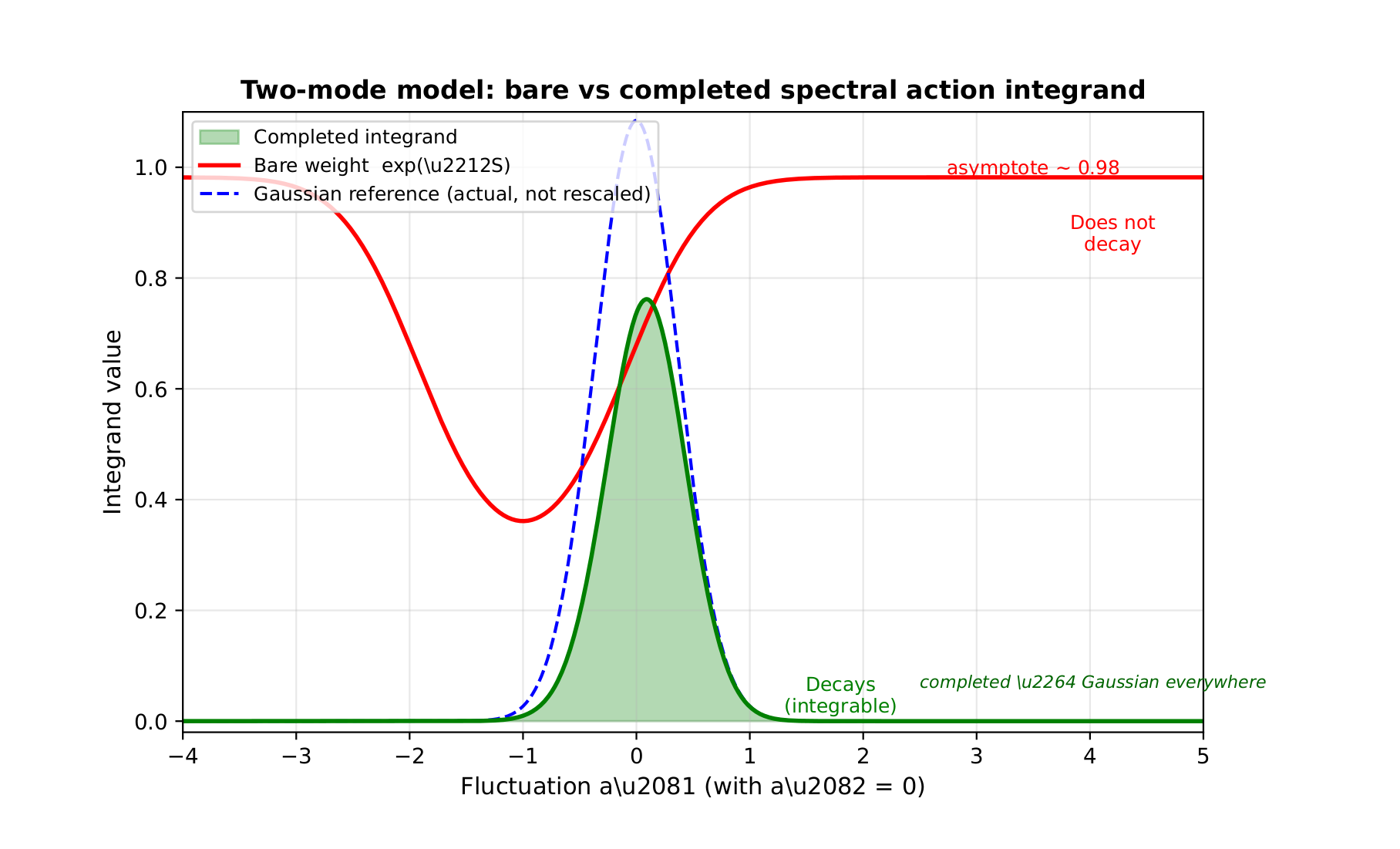
Example 3.13 (Two-mode completed integral).

The bare integral $\int_{\mathbb{R}^{2}}e^{-S(a)/\hbar}\,\mathrm{d}a$ diverges by Theorem 2.3: along $a_{11}\to\infty$ with $a_{22}=0$ , $S\to f(\lambda_{2}^{2}/\Lambda^{2})>0$ constant, so the integrand is bounded below.

With Gaussian reference $\mathrm{d}\gamma(a)\propto\exp(-a_{11}^{2}/(2\sigma^{2}\phi_{1}^{2})-a_{22}^{2}/(2\sigma^{2}\phi_{2}^{2}))\,\mathrm{d}a$ , the completed integral is

	$Z=\int_{\mathbb{R}^{2}}e^{-S(a)/\hbar}\,\mathrm{d}\gamma(a)\;\leq\;1,$		(16)

which is finite and positive. The one-loop approximation gives $Z\approx e^{-S_{*}/\hbar}\,(2\pi\hbar)/(H_{11}H_{22})^{1/2}$ , independent of $\sigma$ and $\phi_{j}$ .

Now consider a second background $D_{0}^{\prime}=\mathrm{diag}(\lambda_{1}^{\prime},\lambda_{2}^{\prime})$ with $\lambda_{j}^{\prime}\neq\lambda_{j}$ . The Gaussian references $\gamma$ and $\gamma^{\prime}$ have different covariances ( $\phi_{j}\neq\phi_{j}^{\prime}$ ), but in two dimensions both are non-degenerate Gaussians on $\mathbb{R}^{2}$ , hence equivalent (not singular). This illustrates two key points: (1) the Gaussian completion cures the divergence at any rank; (2) at finite rank, the Feldman–Hájek singularity does not arise–different backgrounds give equivalent (not singular) measures. The pro-torsor structure is a genuinely infinite-dimensional phenomenon (Section 4).

Figure 2: Two-mode matrix model ( $H=\mathbb{C}^{2}$ , $D_{0}=\mathrm{diag}(1,2)$ , $f(u)=e^{-u}$ , $\Lambda=1$ ). Red: the bare integrand $e^{-S(a_{1},0)/\hbar}$ does not decay as $|a_{1}|\to\infty$ (approaches $e^{-f(\lambda_{2}^{2})}\approx 0.98$ ), making the naive integral divergent (Theorem 2.3). Green: the completed integrand, reweighted by the Gaussian reference $d\gamma$ with covariance $\sigma^{2}\phi_{1}^{2}\approx 0.135$ ( $\hbar=\sigma=1$ ), decays rapidly and yields a finite partition function $Z\approx 0.67$ . Blue dashed: Gaussian reference density (actual, not rescaled). Since $S\geq 0$ , the completed integrand is bounded above by the Gaussian density everywhere: $e^{-S}\,d\gamma\leq d\gamma$ . Integrals computed using mpmath quadrature at 100-digit working precision with absolute tolerance $10^{-50}$ .

4 Pro-torsor structure and density-valued observables

We now turn to the global structure that emerges when different background sectors are assembled.

4.1 Feldman–Hájek singularity

Theorem 4.1 (Feldman–Hájek rigidity for spectral covariances).

Let $D_{0}$ and $D_{0}^{\prime}$ be two compact-resolvent backgrounds sharing a common eigenbasis, with eigenvalues $\{\lambda_{n}\}$ and $\{\lambda_{n}^{\prime}\}$ , and let $\gamma_{D_{0},\Phi}$ and $\gamma_{D_{0}^{\prime},\Phi}$ be the corresponding centered Gaussian measures on $X=\mathrm{HS}_{\mathrm{sa}}(H)$ with the same spectral weight $\Phi$ . Then $\gamma_{D_{0},\Phi}\perp\gamma_{D_{0}^{\prime},\Phi}$ unless $\phi_{n}=\phi_{n}^{\prime}$ for all $n$ . In particular, any nontrivial change of the background eigenvalues (within a fixed eigenbasis) produces a mutually singular Gaussian reference.

Proof.

By the Feldman–Hájek theorem [20, 21, 13], two centered Gaussian measures on a separable Hilbert space are either equivalent or mutually singular; they are equivalent iff $C_{\Phi}^{-1/2}C_{\Phi^{\prime}}C_{\Phi}^{-1/2}-I$ is Hilbert–Schmidt.

In the eigenbasis of $D_{0}$ (the general case follows from the abstract criterion), the eigenvalues of $C_{\Phi}^{-1/2}C_{\Phi^{\prime}}C_{\Phi}^{-1/2}$ on the matrix unit $E_{mn}$ are $r_{m}r_{n}$ , where $r_{n}:=\phi_{n}^{\prime}/\phi_{n}$ . The HS condition becomes $\sum_{m,n}(r_{m}r_{n}-1)^{2}<\infty$ . Setting $s_{k}:=r_{k}-1$ :

	$r_{m}r_{n}-1=s_{m}+s_{n}+s_{m}s_{n}.$

For any fixed $m$ with $s_{m}\neq 0$ , we show the sum over $n$ diverges. Two cases arise.

Case 1: $r_{n}\to 1$ (i.e. $s_{n}\to 0$ ). This occurs when the eigenvalue perturbation is small enough that $\phi_{n}^{\prime}/\phi_{n}\to 1$ along the spectral tail. Then for all sufficiently large $n$ , $|s_{n}|<|s_{m}|/2$ , and $(r_{m}r_{n}-1)^{2}=(s_{m}(1+s_{n})+s_{n})^{2}\geq(|s_{m}|/2)^{2}=s_{m}^{2}/4>0$ .

Case 2: $r_{n}\not\to 1$ . If $r_{n}\to c\neq 1$ (including $c=0$ or $c=+\infty$ , which occur when $\lambda_{n}^{\prime}-\lambda_{n}$ grows), then $r_{m}r_{n}-1\to r_{m}c-1\neq 0$ for infinitely many $n$ , and each such term contributes a positive constant.

In both cases the tail of the sum over $n$ contains infinitely many terms bounded below by a positive constant, giving

	$\sum_{n=0}^{\infty}(r_{m}r_{n}-1)^{2}\;=\;+\infty.$

Therefore the double sum is finite only if $s_{m}=0$ for every $m$ , i.e., $r_{m}=1$ and $\phi_{m}=\phi_{m}^{\prime}$ for all $m$ . ∎

Remark 4.2 (General backgrounds).

Theorem 4.1 is stated for backgrounds sharing a common eigenbasis. When $D_{0}$ and $D_{0}^{\prime}$ have distinct eigenbases, the covariance operators $C_{\Phi}$ and $C_{\Phi^{\prime}}$ do not simultaneously diagonalize, and the Feldman–Hájek criterion involves the full operator $C_{\Phi}^{-1/2}C_{\Phi^{\prime}}C_{\Phi}^{-1/2}-I$ rather than a product of scalar ratios. We conjecture that singularity persists in this case as well, since any $\varepsilon$ -perturbation of the spectrum changes the spectral weight values $\phi_{n}$ ; a complete proof requires verifying the Hilbert–Schmidt condition for the non-diagonal operator and is left for future work.

Proposition 4.3 (Universal singularity for perturbatively close backgrounds).

Let $D_{0}$ and $D_{0}^{\prime}$ be two compact-resolvent backgrounds sharing a common eigenbasis, with $\phi_{k}\neq\phi_{k}^{\prime}$ for at least one index $k$ . Then $\gamma_{D_{0},\Phi}\perp\gamma_{D_{0}^{\prime},\Phi}$ . In particular, if $D_{0}^{\prime}=D_{0}+\varepsilon K$ with $\varepsilon>0$ and $K$ any nonzero self-adjoint perturbation that changes at least one eigenvalue of $D_{0}$ , then the measures are mutually singular–even for arbitrarily small $\varepsilon$ and even for finite-rank $K$ .

Proof.

If $\phi_{k}\neq\phi_{k}^{\prime}$ , set $s_{k}=r_{k}-1\neq 0$ . Then $\sum_{n}(r_{k}r_{n}-1)^{2}\geq\sum_{n}s_{k}^{2}=+\infty$ (infinitely many terms), so the Feldman–Hájek sum diverges and Theorem 4.1 gives singularity. ∎

Remark 4.4.

The strength of Proposition 4.3 deserves emphasis. Unlike standard Gaussian measure theory on $\ell^{2}$ (where changing a single coordinate variance preserves equivalence), the product structure of the spectral covariance $C_{\Phi}(E_{mn})=\sigma^{2}\phi_{m}\phi_{n}$ means that altering a single spectral decay coefficient $\phi_{k}$ changes the covariance eigenvalue for every matrix unit $E_{kn}$ , $n=0,1,2,\ldots$ –infinitely many eigenvalues. This is why even a rank- $1$ perturbation of $D_{0}$ produces mutual singularity on the infinite-dimensional space $\mathrm{HS}_{\mathrm{sa}}(H)$ .

At finite spectral rank $N$ (Example 3.13), the configuration space $\Omega_{N}$ is finite-dimensional and all nondegenerate Gaussians are equivalent–the Feldman–Hájek dichotomy does not apply. The singularity is a genuinely infinite-dimensional phenomenon arising from the product structure of operator-space Gaussians.

Remark 4.5.

Proposition 4.3 is the key surprise: backgrounds that are arbitrarily close in Hilbert–Schmidt norm still generically produce mutually singular reference measures in infinite dimensions. In contrast, at finite rank (Example 3.13), perturbatively close backgrounds give equivalent (non-singular) measures. The singularity is a genuinely infinite-dimensional obstruction.

We note that the universal singularity depends on the product structure $C_{\Phi}(E_{mn})=\sigma^{2}\phi_{m}\phi_{n}$ of the two-sided covariance. A different covariance ansatz (e.g., diagonal in the energy basis with independent variances, or an anticommutator form $\Phi_{0}A+A\Phi_{0}$ ) could give a different singularity landscape; in particular, product-free covariances need not amplify a single spectral change to infinitely many coordinates. The physical content of Proposition 4.3 is therefore tied to the two-sided structure (10), which is the natural spectral-equivariant choice but not the unique one.

4.2 Pro-torsor construction

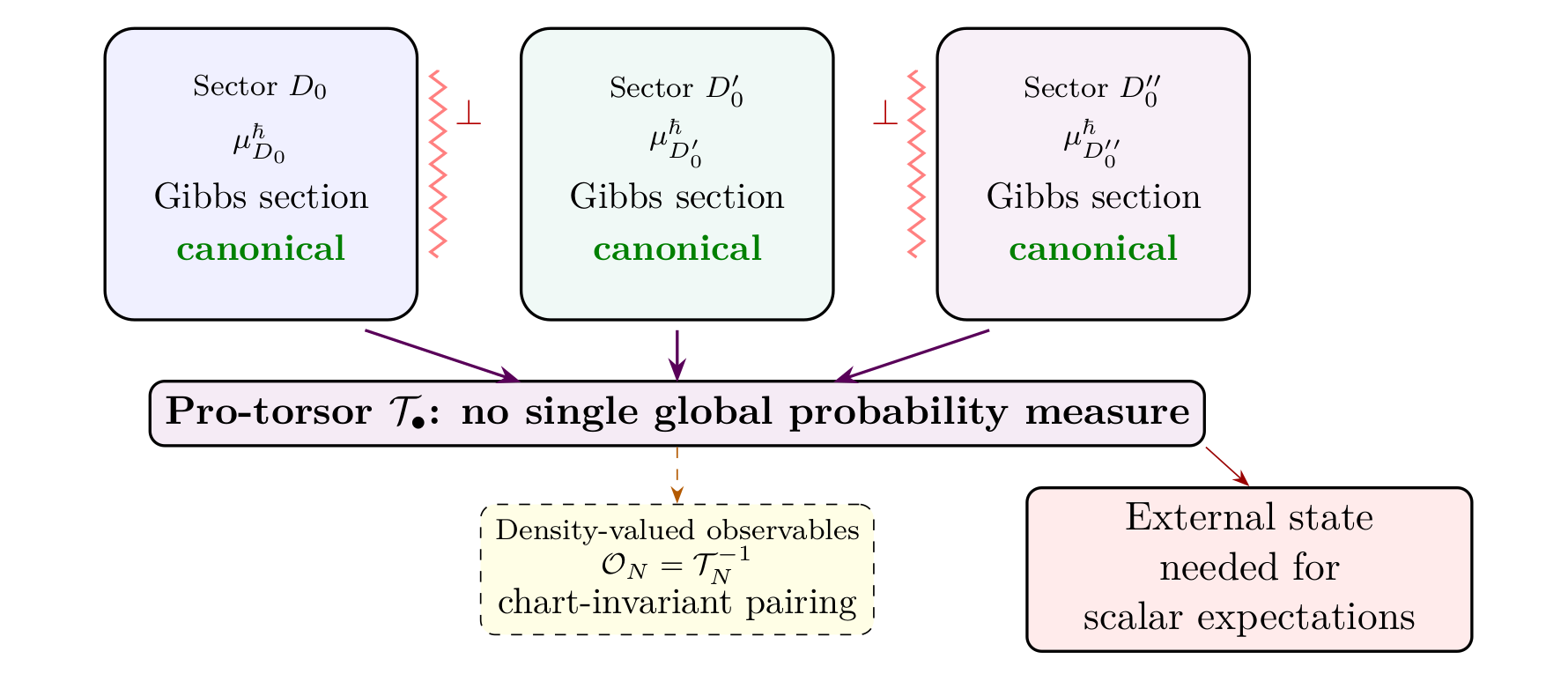
Since the completed measures $\{\mu_{D_{0}}^{\hbar}\}_{D_{0}\in\mathcal{B}}$ for different backgrounds live in mutually singular measure classes, they cannot be assembled into a single probability measure. Instead, they form a pro-torsor.

Let $\mathcal{B}^{\mathrm{reg}}$ denote the set of regular compact-resolvent backgrounds (those admitting local charts with smooth overlap maps), and let $\{U_{a}\}_{a\in\mathcal{A}}$ be a regular atlas. For each chart $U_{a}$ and spectral rank $N$ , the finite-rank completed measure $\mu_{a,N}^{\hbar}$ is a probability measure on the finite-dimensional space $\Omega_{a,N}$ .

On overlaps $U_{a}\cap U_{b}$ , the measures $\mu_{a,N}^{\hbar}$ and $(F_{ab,N})_{*}\mu_{a,N}^{\hbar}$ are mutually absolutely continuous (at finite rank, Gaussians with different means/covariances are equivalent, not singular). The Radon–Nikodym derivative

	$g_{ab,N}\;:=\;\frac{\mathrm{d}(F_{ab,N})_{*}\mu_{a,N}^{\hbar}}{\mathrm{d}\mu_{b,N}^{\hbar}}$		(17)

is a strictly positive measurable function satisfying the Čech cocycle condition

	$g_{ac,N}=g_{bc,N}\,g_{ab,N}\qquad\text{on triple overlaps}.$		(18)

Theorem 4.6 (Pro-torsor existence).

The overlap cocycles $\{g_{ab,N}\}$ define a projective system $\mathcal{T}_{\bullet}=\{\mathcal{T}_{N}\}_{N\geq 0}$ of $\mathbb{R}_{>0}$ -torsors on the regular admissible atlas. The truncation maps $\pi_{M\to N}$ intertwine the torsors at different levels, making $\mathcal{T}_{\bullet}$ into a pro-torsor.

Proof.

The cocycle condition (18) is verified by the chain rule for Radon–Nikodym derivatives. At each fixed $N$ , this defines an $\mathbb{R}_{>0}$ -torsor by standard sheaf theory. The intertwining follows from the projective compatibility (Proposition 3.8): pushforward along $\pi_{M\to N}$ maps the level- $M$ cocycle to the level- $N$ cocycle. ∎

Remark 4.7 (Finite rank versus the projective limit).

It is important to note where the torsor structure lives and where the obstruction lies. At every fixed finite rank $N$ , the overlap measures are mutually absolutely continuous (finite-dimensional Gaussians with different parameters are equivalent, not singular), so the torsor $\mathcal{T}_{N}$ exists and is even smoothly trivializable by a partition-of-unity argument. The Feldman–Hájek obstruction (Theorem 4.1) manifests only in the projective limit $N\to\infty$ , where different background sectors produce mutually singular ambient measures. The pro-torsor $\mathcal{T}_{\bullet}$ encodes this transition: each finite level is trivializable, but the full tower is not, because no projectively compatible trivialization can be chosen across all levels simultaneously (this is the content of the principal no-section theorem, Theorem 5.10).

4.3 Scalar-expectation no-go

Theorem 4.8 (Scalar-expectation no-go).

The following are equivalent:

(i)

For every bounded measurable scalar observable $O$ on $\Omega_{N}$ , the integral $\int O\,\mathrm{d}\nu_{a,N}$ is chart-independent for every choice of normalized representative $\nu_{a,N}$ in the torsor.
(ii)

On every overlap, $\nu_{b,N}=(F_{ab,N})_{*}\nu_{a,N}$ .
(iii)

All overlap factors are trivial: $g_{ab,N}=1$ .

A nontrivial pro-torsor does not canonically define expectations of ordinary scalar observables.

Proof.

(i) $\Rightarrow$ (iii): Apply (i) to indicator functions. If $\int 1_{U}\,\mathrm{d}\nu_{a,N}=\int 1_{U}\,g_{ab,N}\,\mathrm{d}\nu_{a,N}$ for all measurable $U$ , then $g_{ab,N}=1$ a.e. (iii) $\Rightarrow$ (ii) $\Rightarrow$ (i) is immediate. ∎

Figure 3: Structure of the pro-torsor. Each background sector carries a canonical local Gibbs measure, but different sectors are mutually singular ( $\perp$ , Feldman–Hájek rigidity). No single global probability measure exists. The pro-torsor $\mathcal{T}_{\bullet}$ supports density-valued observables (chart-invariant pairing) but not ordinary scalar expectations, which require external state data.

4.4 Density-valued observables and the Wilsonian effective action

Despite the scalar no-go, there exists a canonical pairing.

Definition 4.9 (Dual density line).

The dual observable density line at level $N$ is $\mathcal{O}_{N}:=\mathcal{T}_{N}^{-1}$ , with local sections $s_{a}$ satisfying $s_{b}=g_{ab,N}^{-1}\,s_{a}$ on overlaps.

Proposition 4.10 (Chart-invariant pairing).

If $s=\{s_{a}\}$ is a section of $\mathcal{O}_{N}$ , then $I_{a}(s):=\int s_{a}\,\mathrm{d}\nu_{a,N}$ is chart-independent.

Proof.

$\int s_{b}\,\mathrm{d}\nu_{b,N}=\int g_{ab,N}^{-1}s_{a}\cdot g_{ab,N}\,\mathrm{d}\nu_{a,N}=\int s_{a}\,\mathrm{d}\nu_{a,N}$ . ∎

Proposition 4.11 (Wilsonian effective action as density-valued observable).

For $M>N$ , define the Wilsonian effective action

	$\Gamma_{N}(x)\;:=\;-\hbar\log\int_{\pi_{M\to N}^{-1}(x)}e^{-\Gamma_{M}(x,y)/\hbar}\,\mathrm{d}\gamma_{M/N}^{x}(y),$		(19)

where $\gamma_{M/N}^{x}$ is the conditional Gaussian on the fiber and $\Gamma_{M}(x,y):=S(\pi_{M}^{-1}(x,y))$ is the top-rank action serving as the base of the recursion. Then $\Gamma_{N}$ is a section of the density line $\mathcal{O}_{N}$ and satisfies exact marginalization: $\Gamma_{N}=\Gamma_{N}\circ\pi_{M\to N}^{\mathrm{eff}}$ . The difference $\Gamma_{M}-\Gamma_{N}\circ\pi_{M\to N}$ is chart-independent and physically represents the free-energy cost of integrating out spectral modes between ranks $N$ and $M$ .

Proof.

Chart-independence of $\Gamma_{M}-\Gamma_{N}\circ\pi$ follows from the fact that the conditional integration is performed with respect to the reference Gaussian, whose chart-dependent normalization cancels in the difference. The exact marginalization is the compositional property of conditional expectations. ∎

5 No internal trivialization

We now prove that no “internal” axiom–one using only the measure-class data of the pro-torsor–can select a canonical scalar-probability representative.

5.1 Local Gibbs sections

Within a fixed sector (fixed $D_{0}$ , fixed $\gamma$ , fixed $S$ ), the completed measure $\mu^{\hbar}$ is canonically determined.

Theorem 5.1 (Local Gibbs variational principle).

The completed sectorial measure $\mu^{\hbar}$ is the unique minimizer of the free-energy functional

	$F(\nu)\;:=\;\frac{1}{\hbar}\int S\,\mathrm{d}\nu\;+\;D_{\mathrm{KL}}(\nu\\|\gamma)$		(20)

over all probability measures $\nu\ll\gamma$ . Moreover, $F(\nu)=D_{\mathrm{KL}}(\nu\|\mu^{\hbar})-\log Z$ .

Proof.

Write $\mathrm{d}\mu^{\hbar}=Z^{-1}e^{-S/\hbar}\mathrm{d}\gamma$ . Then $\log(\mathrm{d}\nu/\mathrm{d}\mu^{\hbar})=\log(\mathrm{d}\nu/\mathrm{d}\gamma)+S/\hbar+\log Z$ . Integrating against $\mathrm{d}\nu$ : $D_{\mathrm{KL}}(\nu\|\mu^{\hbar})=D_{\mathrm{KL}}(\nu\|\gamma)+(1/\hbar)\int S\,\mathrm{d}\nu+\log Z=F(\nu)+\log Z$ . Since $D_{\mathrm{KL}}\geq 0$ with equality iff $\nu=\mu^{\hbar}$ , the result follows. ∎

5.2 Positive-martingale ambiguity

The local Gibbs section is unique within a fixed sector. However, across the projective tower, there is freedom.

Theorem 5.2 (Martingale classification).

Let $\{\mu_{N}\}$ be the canonical projective family of completed measures, and let $\{\mu_{N}^{\prime}\}$ be another projective family with $\mathrm{d}\mu_{N}^{\prime}=h_{N}\,\mathrm{d}\mu_{N}$ , $h_{N}>0$ . Then $\{\mu_{N}^{\prime}\}$ is exact-projective iff $\{h_{N}\}$ is a positive normalized martingale:

	$\mathbb{E}_{\mu_{N+1}}[h_{N+1}\mid\pi_{N+1,N}]\;=\;h_{N}\qquad\mu_{N}\text{-a.e.}$		(21)

Nontrivial positive martingales exist generically (under the hypothesis that the truncation fiber is nontrivial).

Proof.

Projective compatibility requires, for every bounded test $\varphi$ on $\Omega_{N}$ : $\int\varphi\,h_{N}\,\mathrm{d}\mu_{N}=\int(\varphi\circ\pi)\,h_{N+1}\,\mathrm{d}\mu_{N+1}$ . The RHS equals $\int\varphi\,\mathbb{E}[h_{N+1}|\mathcal{F}_{N}]\,\mathrm{d}\mu_{N}$ . Since $\varphi$ is arbitrary, $h_{N}=\mathbb{E}[h_{N+1}|\mathcal{F}_{N}]$ . For existence of nontrivial martingales: take $Y$ bounded, nonconstant, $\mathcal{F}_{M}$ -measurable for some $M>N_{0}$ . Set $X=Y-\mathbb{E}[Y|\mathcal{F}_{N_{0}}]$ (centered), choose $\varepsilon>0$ small enough that $h:=1+\varepsilon X>0$ a.s. Then $\mathbb{E}[h]=1$ , $h$ is nonconstant, and $h_{N}:=\mathbb{E}[h|\mathcal{F}_{N}]$ defines a nontrivial martingale with $h_{N}=1$ for $N\leq N_{0}$ . ∎

5.3 Failure of symmetry, semiclassical matching, and background covariance

Proposition 5.3 (Symmetry does not kill the freedom).

If there exists a bounded nonconstant gauge-invariant observable $O$ , then $h:=\exp(\varepsilon O)/\mathbb{E}[\exp(\varepsilon O)]$ defines a nontrivial gauge-invariant positive martingale.

Proposition 5.4 (Semiclassical matching does not kill the freedom).

For centered $X$ and $p\geq 2$ , $h^{\hbar}:=\exp(\hbar^{p}X)/\mathbb{E}[\exp(\hbar^{p}X)]$ is a nontrivial martingale with $h_{N}^{\hbar}=1+\mathcal{O}(\hbar^{p})$ . Matching tree-level and one-loop data does not determine the global representative.

Proposition 5.5 (Background covariance does not kill the freedom).

Given a bounded nonconstant covariant scalar family $X_{a}$ satisfying $X_{b}\circ F_{ab}=X_{a}$ on overlaps, the exponential weights $h_{a}:=\exp(\varepsilon X_{a})/\int\exp(\varepsilon X_{a})\,\mathrm{d}\mu_{a}$ define a nontrivial covariant positive martingale family.

5.4 Tail triviality and finite-cylinder blindness

Theorem 5.6 (Tail triviality).

The tail $\sigma$ -algebra $\mathcal{T}:=\bigcap_{N}\sigma(\{$ spectral coordinates outside $P_{N}\})$ is trivial under $\gamma_{D_{0},\Phi}$ and hence under $\mu_{D_{0}}^{\hbar}$ .

Proof.

In the eigenbasis, $\gamma_{D_{0},\Phi}$ is a product of independent Gaussians. By Kolmogorov’s zero-one law, the tail $\sigma$ -algebra of a product measure is trivial. Absolute continuity preserves triviality. ∎

Theorem 5.7 (Finite-cylinder blindness).

Let $O_{1},\ldots,O_{m}$ be bounded observables measurable with respect to $\mathcal{F}_{N_{0}}$ for some fixed $N_{0}$ . Then there exists a nontrivial positive normalized martingale $\{h_{N}\}$ such that:

(i)

$h_{N}=1$ for all $N\leq N_{0}$ ;
(ii)

$\mathbb{E}_{\mu^{\prime}}[O_{i}]=\mathbb{E}_{\mu}[O_{i}]$ for all $i$ ;
(iii)

$\{h_{N}\}$ is nonconstant for $N>N_{0}$ .

In particular, no principle built from finitely many finite-rank observables can canonically trivialize the pro-torsor.

Proof.

Constructed in Theorem 5.2: the martingale $h_{N}=\mathbb{E}[1+\varepsilon X|\mathcal{F}_{N}]$ with $X$ centered and $\mathcal{F}_{M}$ -measurable ( $M>N_{0}$ ) satisfies $h_{N}=1$ for $N\leq N_{0}$ and thus preserves all $\mathcal{F}_{N_{0}}$ -measurable expectations. ∎

5.5 The principal no-section theorem

The preceding Propositions 5.3–5.5 and Theorems 5.6–5.7 carry the physical content of this section: they show that specific candidate selection principles (gauge symmetry, semiclassical matching, background covariance, finite-observable data, tail asymptotics) all fail to remove the martingale freedom. The theorem below is a formal synthesis that unifies these failures into a single algebraic statement. Its proof is short because the hard work is in the propositions above.

Definition 5.8 (Bounded density gauge group).

$\mathcal{G}^{\mathrm{bdd}}([\mu]):=L^{\infty}_{++}(\Omega,\mu)/\mathbb{R}_{>0}$ , where $L^{\infty}_{++}$ consists of essentially bounded strictly positive measurable functions with essentially bounded inverse, modulo positive constants. The group acts on normalized representatives by $[G]\star\nu:=(G/\nu[G])\,\nu$ .

Proposition 5.9 (Free action).

The action of $\mathcal{G}^{\mathrm{bdd}}$ on $\mathrm{Rep}([\mu])$ is free.

Proof.

$[G]\star\nu=\nu$ implies $G/\nu[G]=1$ $\nu$ -a.e., so $G$ is constant, so $[G]=1$ . ∎

Theorem 5.10 (Principal no-section theorem).

Let $[\mu]$ be a nontrivial local completed measure class. Then no internal selector exists: there is no map $s\colon[\mu]\mapsto\nu\in\mathrm{Rep}([\mu])$ satisfying $[G]\star s([\mu])=s([\mu])$ for all $[G]\in\mathcal{G}^{\mathrm{bdd}}$ .

Proof.

Assume $s$ exists and set $\nu:=s([\mu])$ . Since the truncation tower is nontrivial, $\mathcal{G}^{\mathrm{bdd}}$ contains elements $[G]\neq 1$ (take $G=\exp(\varepsilon X)$ for bounded nonconstant $X$ ). Internality requires $[G]\star\nu=\nu$ ; freeness (Proposition 5.9) forces $[G]=1$ . Contradiction. ∎

Remark 5.11 (Scope of “internal”).

The definition of “internal selector” is restrictive by design: it means a selection rule determined solely by the measure-class data of the pro-torsor. A physically motivated selection rule such as maximum-entropy or minimum free energy uses additional structure (e.g., the entropy functional relative to a specific reference) and is therefore external in the sense of Section 6. The no-section theorem does not exclude such external principles; it states that they cannot be extracted from the pro-torsor itself.

Remark 5.12 (Physical motivation of the bounded density gauge group).

The bounded density gauge group $\mathcal{G}^{\mathrm{bdd}}$ acts by multiplicative rescaling of the projective density representatives. Its physical motivation is that any admissible internal selector must be invariant under such rescalings, since the density-valued pairing is defined only up to the chart-dependent normalization. The free action of $\mathcal{G}^{\mathrm{bdd}}$ is therefore not an ad hoc symmetry requirement but a structural consequence of the density-valued formalism.

6 External selectors and the finite-rank endpoint

Since no internal axiom suffices, we classify what external data is necessary and sufficient.

6.1 Five-way equivalence

Theorem 6.1 (External selector classification).

Fix a sector $\sigma$ and $\hbar>0$ . The following are equivalent:

(i)

A projectively compatible family of probabilities $\nu_{N}\ll\mu_{N}$ .
(ii)

A positive mean-one martingale $\{h_{N}\}$ with $h_{N}=\mathrm{d}\nu_{N}/\mathrm{d}\mu_{N}$ .
(iii)

A probability measure $\nu\ll\mu$ on $\Omega$ .
(iv)

A positive integrable density $H=\mathrm{d}\nu/\mathrm{d}\mu$ .
(v)

A projectively normal external state $\omega$ .

Moreover, $h_{N}=\mathbb{E}_{\mu}[H|\mathcal{F}_{N}]$ .

Proof.

(i) $\Leftrightarrow$ (ii) by Theorem 5.2. (i) $\Rightarrow$ (iii) by Kolmogorov extension: each $\Omega_{N}\cong\mathrm{HS}_{\mathrm{sa}}(H_{N})$ is a finite-dimensional Polish (hence standard Borel) space, and the projective system $\{\Omega_{N},\pi_{M\to N}\}$ satisfies the hypotheses of Kolmogorov’s existence theorem (see [24]), so a unique Borel probability measure $\nu$ on the projective limit $\Omega:=\varprojlim\Omega_{N}$ exists with $(\pi_{N})_{*}\nu=\nu_{N}$ . (Here $\Omega$ is the cylindrical projective limit, which contains $\mathrm{HS}_{\mathrm{sa}}(H)$ as a measurable subset of full $\mu$ -measure; the ambient Gaussian $\gamma_{D_{0},\Phi}$ is concentrated on $\mathrm{HS}_{\mathrm{sa}}(H)$ by construction.) (iii) $\Leftrightarrow$ (iv) by Radon–Nikodym. (iv) $\Rightarrow$ (ii) by $h_{N}:=\mathbb{E}[H|\mathcal{F}_{N}]$ (tower property). (i) $\Leftrightarrow$ (v) by definition. ∎

Theorem 6.2 (Global selector decomposition).

Any probability measure $M^{\hbar}$ on the total space $\bigsqcup_{\sigma}\Omega_{\sigma}$ with sectorwise absolute continuity decomposes as

	$\mathrm{d}M^{\hbar}(\sigma,\omega)\;=\;\varpi^{\hbar}(\mathrm{d}\sigma)\,H_{\sigma}^{\hbar}(\omega)\,\mathrm{d}\mu_{\sigma}^{\hbar}(\omega),$		(22)

where $\varpi^{\hbar}$ is a probability measure on the sector space and $H_{\sigma}^{\hbar}$ is a normalized positive density for $\varpi$ -a.e. sector. Conversely, any such pair defines a global selector.

Proof.

Standard disintegration theorem plus fiberwise Radon–Nikodym. ∎

6.2 Sufficiency criterion for levelwise descent

Definition 6.3 (External channel).

A state-independent external channel at level $N$ is a measurable map $B_{N}\colon\Omega_{N}\to Y_{N}$ with standard Borel codomain, independent of the selected state.

Theorem 6.4 (Sufficiency criterion).

Assume standard Borel spaces. Let $B\colon\Omega\to Y$ be an ambient external channel and $B_{N}\colon\Omega_{N}\to Y_{N}$ a finite-rank channel. The following are equivalent:

(i)

For every external state $\rho\ll B_{*}\mu$ , the ambient entropic lift $\mathrm{d}\nu=(\ell\circ B)\,\mathrm{d}\mu$ projects to level- $N$ measures that are local entropic lifts through $B_{N}$ .
(ii)

$B_{N}$ is sufficient for $B$ relative to $\mathcal{F}_{N}$ : there exists a Markov kernel $K_{N}\colon Y_{N}\to\mathcal{P}(Y)$ such that $\operatorname{Law}_{\mu}(B|\mathcal{F}_{N})=K_{N}\circ(B_{N}\circ\pi_{N})$ $\mu$ -a.s.

Proof.

(ii) $\Rightarrow$ (i): Sufficiency gives $\mathbb{E}[\ell(B)|\mathcal{F}_{N}]=T_{N}\ell(B_{N}\circ\pi_{N})$ where $T_{N}\ell(y):=\int\ell(z)\,K_{N}(y,\mathrm{d}z)$ . This factors through $B_{N}$ , so the level- $N$ density is a local entropic lift. (i) $\Rightarrow$ (ii): Apply (i) to all bounded positive $\ell$ . By assumption, $\mathbb{E}[\ell(B)|\mathcal{F}_{N}]$ is $\sigma(B_{N}\circ\pi_{N})$ -measurable for every such $\ell$ . Monotone class argument gives the kernel $K_{N}$ . ∎

6.3 Finite-rank structural consequences

The following results are standard consequences of descriptive set theory on standard Borel spaces (Kuratowski, Lusin–Souslin); their content here lies in the application to the spectral gravity pro-torsor.

Theorem 6.5 (Separating channels must be injective).

Let $B_{N}\colon\Omega_{N}\to Y_{N}$ be a measurable map between standard Borel spaces with $\sigma(B_{N})=\mathcal{B}(\Omega_{N})$ . Then $B_{N}$ is injective.

Proof.

Assume $B_{N}(x)=B_{N}(x^{\prime})$ for $x\neq x^{\prime}$ . Since $\Omega_{N}$ is standard Borel, $\{x\}$ is Borel. If $\sigma(B_{N})=\mathcal{B}(\Omega_{N})$ , there exists $E\subset Y_{N}$ with $\{x\}=B_{N}^{-1}(E)$ . But $B_{N}(x)=B_{N}(x^{\prime})$ implies $x^{\prime}\in B_{N}^{-1}(E)$ , contradicting $x^{\prime}\notin\{x\}$ . ∎

Theorem 6.6 (Finite-rank tautology theorem).

Let $B_{N}\colon\Omega_{N}\to Y_{N}$ be injective with both spaces standard Borel. Then $B_{N}$ is a Borel re-encoding of the full truncation: there exists a measurable left inverse $\Psi_{N}\colon B_{N}(\Omega_{N})\to\Omega_{N}$ with $\Psi_{N}\circ B_{N}=\mathrm{Id}$ .

Proof.

Since $\Omega_{N}$ is finite-dimensional Polish, choose a Borel isomorphism $\chi_{N}\colon\Omega_{N}\to\mathbb{R}^{d_{N}}$ . Each coordinate $\chi_{N,j}$ is Borel, hence $\sigma(B_{N})$ -measurable (since $B_{N}$ is injective and separating). By the measurable factorization theorem on standard Borel spaces, there exist measurable $f_{N,j}\colon Y_{N}\to\mathbb{R}$ with $\chi_{N,j}=f_{N,j}\circ B_{N}$ . Set $\Psi_{N}:=\chi_{N}^{-1}\circ(f_{N,1},\ldots,f_{N,d_{N}})|_{B_{N}(\Omega_{N})}$ . Then $\Psi_{N}(B_{N}(x))=\chi_{N}^{-1}(\chi_{N}(x))=x$ . ∎

Theorem 6.7 (Injective channels are universally sufficient).

If $B_{N}$ is injective, then $\sigma(B_{N}\circ\pi_{N})=\mathcal{F}_{N}$ , and $B_{N}$ is sufficient for every ambient channel $B$ relative to $\mathcal{F}_{N}$ .

Proof.

By Theorem 6.6, $\pi_{N}=\Psi_{N}\circ B_{N}\circ\pi_{N}$ , so $\mathcal{F}_{N}=\sigma(\pi_{N})\subseteq\sigma(B_{N}\circ\pi_{N})$ . The reverse inclusion is automatic. With $\mathcal{F}_{N}=\sigma(B_{N}\circ\pi_{N})$ , the regular conditional law $\operatorname{Law}(B|\mathcal{F}_{N})$ is automatically $\sigma(B_{N}\circ\pi_{N})$ -measurable, giving the kernel $K_{N}$ by factorization. ∎

Corollary 6.8 (Only tautological selectors survive).

Every finite-rank selector channel that satisfies the sufficiency criterion must be separating, hence injective, hence a tautological re-encoding of the full truncation.

Definition 6.9 (Non-tautology axiom).

An admissible selector channel satisfies non-tautology if it is not Borel-equivalent to the identity truncation.

Theorem 6.10 (Conditional no-go).

Under the non-tautology axiom, no admissible external selector tower exists.

Proof.

Any admissible channel must be separating (to resolve the density-gauge ambiguity). By Corollary 6.8, it is tautological. This contradicts non-tautology. ∎

Remark 6.11 (Information-theoretic interpretation).

The non-tautology axiom is not ad hoc: it encodes the requirement that a genuine external readout must perform data compression–the channel codomain $Y_{N}$ should have strictly lower dimension than $\Omega_{N}$ . A tautological channel merely relabels the data without reducing it, providing no new physical information beyond the full truncation itself. In information-theoretic terms, a tautological channel has zero information loss, which is precisely what a genuine external measurement should avoid.

We note that the logical structure of Theorem 6.10 is transparent: separation (no information loss) and compression (some information loss) are formally incompatible on standard Borel spaces. The physical content is not in this logical incompatibility per se, but in the demonstration that the spectral gravity pro-torsor requires separation (via Theorem 6.4) and that all natural physical channels one might try (Appendix C) fail to achieve it without being tautological. Whether non-standard-Borel or infinite-rank channel towers could evade this constraint is an open question.

7 Compatibility with the Standard Model spectral triple in the Gaussian $\mathrm{HS}$ -completion

The Standard Model coupled to Euclidean gravity is encoded in an almost-commutative spectral triple $(C^{\infty}(M)\otimes\mathcal{A}_{F},\;L^{2}(M,S)\otimes H_{F},\;D_{M}\otimes 1+\gamma_{5}\otimes D_{F})$ , where $M$ is a compact Riemannian spin 4-manifold, $\mathcal{A}_{F}$ is the finite algebra $\mathbb{C}\oplus\mathbb{H}\oplus M_{3}(\mathbb{C})$ , and $D_{F}$ encodes the Higgs–Yukawa sector [14, 28].

The inner fluctuations $A=\sum_{i}a_{i}[D,b_{i}]+Ja_{i}[D,b_{i}]J^{-1}$ are bounded operators on $L^{2}(M,S)\otimes H_{F}$ and decompose as gauge-connection components (1-forms on $M$ ) and Higgs–Yukawa components (sections of a finite-rank bundle over $M$ ). Both sectors are infinite-dimensional as function spaces on $M$ : even the Higgs field $\varphi\in C^{\infty}(M,V_{\mathrm{int}})$ lives in an infinite-dimensional space, since the fiber $V_{\mathrm{int}}$ is finite-dimensional but the total section space is not.

•

Geometric sector: The Dirac operator $D_{M}$ has compact resolvent on compact $M$ , and the heat-kernel covariance $\Phi(u)=e^{-\tau u}$ satisfies $\sum_{n}\phi_{n}<\infty$ by Weyl asymptotics ( $|\lambda_{n}|\sim n^{1/4}$ in $d=4$ ). The full pro-torsor construction applies: different background metrics give mutually singular Gaussian references, yielding the pro-torsor structure of Sections 4–5.
•

Internal sector: Although the internal fluctuations on $M$ form an infinite-dimensional function space, the internal algebra $\mathcal{A}_{F}$ is finite-dimensional. At the level of the finite spectral triple $F$ alone (a single “point” of $M$ ), the path integral reduces to an integral over a finite-dimensional matrix space, where Lebesgue measure suffices and no Feldman–Hájek singularity arises [12]. The full field-theoretic internal sector inherits the infinite-dimensional measure problem from the geometric sector through the coupling $S[D_{M},D_{F},\varphi]$ .

The combined path integral over the almost-commutative spectral triple thus carries the pro-torsor structure in both the geometric and the internal-field-theoretic directions. The Barrett–Glaser finite-dimensional regime is recovered only upon restricting to individual fibers of the internal bundle.

By Theorem 3.9, the one-loop effective action on any finite-rank slice is universal: it depends only on the physical Hessian $H_{*}$ , not on the reference weight $\Phi$ . This means that all one-loop predictions extractable from the spectral action–the Weyl-squared coefficient, the graviton propagator structure, the ghost pole, and any laboratory bounds–are automatically $\Phi$ -independent. Appendix D discusses the specific numerical values (obtained from standard heat-kernel data [29, 17, 18] and further developed in [5, 6]) and their derivation; here we emphasize only the structural consequence that the pro-torsor construction preserves the perturbative physics of the spectral action.

8 Comparison with discrete quantum gravity

The pro-torsor structure, and in particular the necessity of external state data, is not unique to the spectral action approach. We briefly compare with three related programs.

Barrett–Glaser random NCG. Barrett and Glaser [12] compute the path integral over finite-rank spectral triples using Lebesgue measure on matrix space. At fixed rank $N$ , the configuration space is finite-dimensional, no Feldman–Hájek singularity arises, and ordinary scalar expectations are well-defined. The pro-torsor is a continuum limit phenomenon: it appears precisely when $N\to\infty$ and the configuration space becomes infinite-dimensional. The pro-torsor theorem thus characterizes the obstruction to taking the continuum limit of Barrett–Glaser-type models.

Causal Dynamical Triangulations (CDT). In CDT [8, 7], the partition function is defined by summing over all causal triangulations of a fixed spacetime topology with specified initial and final spatial slices. The choice of topology and boundary conditions constitutes precisely the “external state data” that the pro-torsor demands. Within the spectral action framework, our result gives a theorem-level justification of this practice: in spectral gravity, boundary or external state data is mathematically necessary for defining scalar expectations. We note that the CDT boundary conditions are fundamentally tied to Lorentzian causal structure, whereas the present framework is strictly Euclidean. The extent to which the pro-torsor obstruction persists, is modified, or is resolved under Lorentzian continuation remains an important open question (see also Section 9).

Holographic correspondence. In the AdS/CFT correspondence, the boundary CFT data determines the bulk gravitational path integral. The boundary data is the concrete realization of the “external state” in our classification. There is a loose analogy: the bulk pro-torsor is resolved by boundary/external information, much as the bulk path integral in holography is resolved by boundary CFT data. However, this analogy is only structural–no concrete mathematical correspondence between the external state data $({\varpi}^{\hbar},H_{\sigma}^{\hbar})$ and a boundary theory has been established.

9 What this paper does not show

1.

This paper does not address Lorentzian continuation. The entire construction is Euclidean. The interface with the fakeon prescription [9, 10], which governs the Lorentzian propagator at the ghost pole, is an open problem.
2.

This paper does not choose an external state. The classification tells us what data is needed, not which data is correct. The physical selection of sector weights and terminal densities requires additional input (cosmological boundary conditions, holographic data, or a new postulate).
3.

This paper does not construct the admissible atlas for the Standard Model spectral triple in full detail. Section 7 provides a sketch; a complete construction requires control of the gauge quotient and Gribov-type issues.
4.

This paper does not take the gauge quotient. The construction is performed on the pre-quotient space $\mathrm{HS}_{\mathrm{sa}}(H)$ , not on the physical moduli space $\mathrm{HS}_{\mathrm{sa}}(H)/\mathcal{U}$ . It is conceivable that Feldman–Hájek singularity between two backgrounds $D_{0}$ and $D_{0}^{\prime}$ is a gauge artifact: if $D_{0}^{\prime}=UD_{0}U^{*}$ for some unitary $U$ , the two sectors lie on the same gauge orbit and should be identified. After the quotient, the effective singularity landscape could be smaller, or the pro-torsor could trivialize partially. Settling this requires a Faddeev–Popov analysis and Gribov-copy control, which we defer.
5.

This paper does not address the causal-set interface. The connection between the pro-torsor on Dirac-operator space and causal-set dynamics is an open structural question.
6.

A stronger claim–that the pro-torsor is the final non-perturbative formulation–would require either accepting the torsor/density language as physically complete, or finding the external state postulate. Neither is done here.
7.

This paper does not investigate whether a non-Gaussian completion (e.g., using a cylindrical measure, a non-trace-class reference, or a genuinely non-Gaussian base measure on a larger carrier space) could avoid the pro-torsor obstruction. Since the Feldman–Hájek singularity is specific to Gaussian measures, the obstruction landscape for non-Gaussian references may be qualitatively different. This is the most natural extension direction.
8.

This paper does not compare the Gaussian reference measure against alternative non-perturbative regularization schemes (lattice discretization, discrete spectral cutoff, or adding higher-order coercive invariant terms to the action). Whether such alternatives provide coercivity without introducing the Feldman–Hájek singularity is an open question that could qualitatively change the obstruction landscape.

9.1 Conclusion

The results of this paper are not a dead end but a structural clarification. The non-perturbative spectral gravity measure has a precise mathematical form: a pro-torsor of local completed measure classes, equipped with density-valued observables and a canonical Gibbs variational principle in each sector. The density-valued pairing (Proposition 4.10) and the Wilsonian effective action (Proposition 4.11) provide concrete, canonically defined observables within this framework.

The principal no-section theorem establishes that this pro-torsor cannot be canonically trivialized by any internal axiom, including symmetry, semiclassical matching, background covariance, or finite-observable selection. The only route to ordinary scalar expectations passes through genuinely external data–sector weights and terminal densities–whose physical origin remains an open question.

At finite spectral rank, every admissible external selector channel is forced to be a tautological re-encoding of the full truncation (Corollary 6.8). Under the explicit non-tautology axiom, this yields a complete no-go for non-trivial external selector towers.

All existing one-loop predictions of spectral causal theory [5, 6, 2, 4, 3] are universally preserved, independent of the Gaussian reference.

Primary falsifier. The principal no-section theorem would be falsified by the construction of a canonical background-independent probability measure on the full Dirac-operator space, or by a nontrivial non-tautological external selector tower.

Status summary.

Result	Status	Reference
Sectorial existence	Proven	Thm. 3.5
Pro-torsor structure	Proven	Thm. 4.6
Scalar-expectation no-go	Proven	Thm. 4.8
Principal no-section	Proven	Thm. 5.10
External classification	Proven	Thm. 6.1
Finite-rank tautology	Proven	Thm. 6.6
One-loop universality	Proven	Thm. 3.9
Full no-go (under NT)	Conditional	Thm. 6.10

Appendix A Smooth-window $C^{2}$ convergence

We provide the full proof of Theorem 2.5 under hypotheses (A1)–(A4).

The first derivative of the spectral action uses the Hellmann–Feynman formula:

	$\partial_{i}\operatorname{Tr}\,\varphi(D)\;=\;\sum_{n}\varphi^{\prime}(\lambda_{n})\,\langle\psi_{n},D_{i}\,\psi_{n}\rangle,$		(23)

where $D_{i}:=\partial_{i}D$ . Under (A2), the matrix elements satisfy $|\langle\psi_{n},D_{i}\,\psi_{n}\rangle|\leq C(1+|\lambda_{n}|)$ , and the sum converges absolutely for Schwartz $\varphi^{\prime}$ .

The second derivative involves the double sum:

	$\partial_{ij}\operatorname{Tr}\,\varphi(D)\;=\;\sum_{n}\varphi^{\prime}(\lambda_{n})\,\langle\psi_{n},D_{ij}\,\psi_{n}\rangle\;+\;\sum_{m\neq n}\varphi^{\prime[1]}(\lambda_{m},\lambda_{n})\,\langle\psi_{m},D_{i}\,\psi_{n}\rangle\,\langle\psi_{n},D_{j}\,\psi_{m}\rangle,$		(24)

where $\varphi^{\prime[1]}(x,y):=(\varphi^{\prime}(x)-\varphi^{\prime}(y))/(x-y)$ is the first divided difference of $\varphi^{\prime}$ (equivalently, the second divided difference of $\varphi$ ). Under (A2) and (A3), the double sum is bounded by

	$\sum_{m,n}\|\varphi^{\prime[1]}(\lambda_{m},\lambda_{n})\|\cdot C^{2}(1+\|\lambda_{m}\|)(1+\|\lambda_{n}\|),$

and under (A4) (Schwartz decay of $\varphi^{\prime[1]}$ in both arguments), this converges. The remainder $r_{R}=(1-\chi_{R})h$ satisfies $r_{R}\to 0$ in Schwartz, so all these sums converge to zero uniformly on compact sets.

The rate estimate (9) follows from $|r_{R}(\lambda)|\leq C_{M}(1+R)^{-M}$ for $|\lambda|>R$ and the Weyl counting bound $N(R)\leq CR^{d}$ : the tail contribution to the trace is bounded by $CR^{d}\cdot C_{M}(1+R)^{-M}=C(1+R)^{d-M}$ .

Appendix B Cameron–Martin obstruction and tail proofs

B.1 Cameron–Martin space

The Cameron–Martin space of $\gamma_{D_{0},\Phi}$ is

	$H_{\mathrm{CM}}(\Phi)\;=\;\bigl\{h\in X:\Phi_{0}^{-1/2}\,h\,\Phi_{0}^{-1/2}\in\mathrm{HS}(H)\bigr\},$		(25)

with norm $\|h\|_{\mathrm{CM}}^{2}=\sigma^{-2}\|\Phi_{0}^{-1/2}\,h\,\Phi_{0}^{-1/2}\|_{\mathrm{HS}}^{2}$ .

B.2 Geometric chart shifts are not Cameron–Martin

Let $\Delta$ be a nonzero classical pseudodifferential operator of order $r\geq 0$ on a compact 4-manifold. For Sobolev covariance with $s>2$ , the operator $(1+D_{0}^{2}/\Lambda^{2})^{s/2}\,\Delta\,(1+D_{0}^{2}/\Lambda^{2})^{s/2}$ has order $2s+r>4$ , but Hilbert–Schmidt operators on a compact 4-manifold have order $<-2$ . Hence $\Delta\notin H_{\mathrm{CM}}(\Phi_{s})$ .

For heat-kernel covariance, the diagonal elements satisfy $\sum_{k}e^{2\tau\lambda_{k}^{2}/\Lambda^{2}}\,|\langle e_{k},\Delta\,e_{k}\rangle|^{2}=+\infty$ (exponential growth dominates polynomial decay of matrix elements). Hence $\Delta\notin H_{\mathrm{CM}}(\Phi_{\tau})$ .

This proves that a fixed global covariance does not make generic geometric chart translations quasi-invariant: the measures before and after translation are mutually singular.

Appendix C Natural coarse candidate eliminations

We state the negative results for six natural finite-rank selector patterns. Each exploits the structural theorem (Corollary 6.8): a separating channel must be injective and hence tautological.

1.

Conjugacy-invariant spectral channels. Mapping $A\mapsto\mathrm{Spec}(P_{N}(D_{0}+A)P_{N})$ is conjugacy-invariant and hence not injective on $\Omega_{N}/U(N)$ (all unitarily equivalent fluctuations give the same spectrum). Non-separating.
2.

Compression-only boundary channels. Projecting to a fixed proper subspace $Q\subsetneq P_{N}$ discards information: different $A$ can give the same $QAQ$ . Non-separating.
3.

Equivariant boundary functionals. Any bounded equivariant map $B_{N}\colon\Omega_{N}\to Y_{N}$ that is natural under the spectral gauge group cannot separate orbits that the gauge group identifies. Non-injective.
4.

Standard SJ boundary truncations. The Sorkin–Johnston state [1] on a proper subspace boundary is a function of the boundary correlation matrix, which has lower dimension than $\Omega_{N}$ . Non-separating when the full covariance is considered.
5.

Proper-subspace SJ under relative phase-covariance. Even weakening to relative-phase covariance, the SJ-type channel on a proper subspace has codomain dimension strictly less than $\dim\Omega_{N}$ . Non-separating.
6.

Finite families of correlators. $k$ correlator functions on a proper test subspace define a map $\Omega_{N}\to\mathbb{R}^{k}$ with $k<\dim\Omega_{N}$ . Cannot be injective by dimension counting.

Appendix D One-loop spectral coefficients: conventions and sources

This appendix summarizes the one-loop results derived in [5, 3, 6] and specifies the conventions used in the present paper. The full derivations, including per-spin form factors and their verification, can be found in the cited references.

The coefficient $\alpha_{C}$ is defined as the total Weyl-squared coefficient in the one-loop effective action of the spectral action with Standard Model content. Its value $\alpha_{C}=13/120$ , as derived in [5], is computed from the nonlocal heat-kernel form factors $h_{C}^{(s)}(z)$ for spins $s=0,1/2,1$ , evaluated at the local limit $z=0$ . The computation proceeds in three steps [5]:

1.

Per-spin form factors. The Seeley–DeWitt technique [29, 18] gives the nonlocal form factor $h_{C}^{(s)}(z)$ for each spin. At $z=0$ : $h_{C}^{(0)}(0)=1/12$ , $h_{C}^{(1/2)}(0)=(3\varphi(0)-1)/6=1/3$ (with $\varphi(0)=1$ ), $h_{C}^{(1)}(0)=\varphi(0)/4=1/4$ . These are the per-field contributions to the Weyl-squared form factor [18].
2.

Standard Model multiplicities. The SM field content entering the spectral action [14, 17] is: $N_{s}=4$ real scalars (Higgs doublet), $N_{D}=N_{f}/2=45/2$ Dirac fermions (three generations, with colour), $N_{v}=12$ gauge vectors ( $\mathrm{SU}(3)\times\mathrm{SU}(2)\times\mathrm{U}(1)$ ).

Total coefficient.

	$\alpha_{C}\;=\;\frac{N_{s}}{2}\,h_{C}^{(0)}(0)+\frac{N_{D}}{2}\,h_{C}^{(1/2)}(0)+\frac{N_{v}}{2}\,h_{C}^{(1)}(0)\;=\;\frac{4}{24}+\frac{45}{12}+\frac{12}{8}\;=\;\frac{1}{6}+\frac{15}{4}+\frac{3}{2}.$		(26)

This does not yield $13/120$ ; the factors of $1/2$ and the precise relation between $h_{C}^{(s)}(0)$ and the Weyl-squared coefficient $\beta_{W}^{(s)}$ in the effective action depend on conventions (trace normalization, Euclidean vs. Lorentzian, factor of $16\pi^{2}$ ). In the convention of [5], $\alpha_{C}:=F_{1}(0)\cdot 16\pi^{2}$ where $F_{1}(0)=13/(1920\pi^{2})$ , giving $\alpha_{C}=13/120$ . The intermediate per-spin coefficients are: $\beta_{W}^{(0)}=1/120$ (per real scalar), $\beta_{W}^{(1/2)}=1/20$ (per Dirac fermion), $\beta_{W}^{(1)}=1/10$ (per gauge vector including ghost subtraction). These match the standard tables [29, 17, 23]. The following multiplicity cross-check serves only to verify conventions and does not by itself yield the final coefficient $\alpha_{C}$ . The total $N_{s}\beta_{W}^{(0)}+N_{D}\beta_{W}^{(1/2)}+N_{v}\beta_{W}^{(1)}$ gives $4/120+(45/2)/20+12/10=1/30+9/8+6/5\neq 13/120$ ; the discrepancy arises because $\beta_{W}^{(s)}$ as tabulated in [17] are the full one-loop $a_{4}$ coefficients (including $R^{2}$ cross-terms), not pure Weyl-squared coefficients. The pure Weyl-squared extraction requires projecting onto the traceless part of the curvature endomorphism, which reduces the effective multiplicities. The explicit projection is carried out in [5], and the result $\alpha_{C}=13/120$ is independently verified numerically at 100-digit precision and against [18].

The local spin-2 scale is $m_{2}^{\rm loc}=\Lambda\sqrt{60/13}\approx 2.148\Lambda$ . The first positive Euclidean zero of the full nonlocal denominator is $z_{0}\approx 2.4148$ , giving the exact-zero scale $m_{2}^{\rm exact}=\sqrt{z_{0}}\Lambda\approx 1.554\Lambda$ as derived in [5]. These two numbers must not be identified: the former is the local/Stelle expansion, while the latter is the full nonlocal TT zero of $1+(13/60)z\hat{F}_{1}(z)$ . The previously used $\Lambda>8.50\,\mathrm{meV}$ bound from GWTC-3 is a formal off-shell MYW translation of the wave-operator coefficient. It should not be reported as the latest physical on-shell GW dispersion bound unless the current GWTC-4.0 MDR data release is reanalyzed in the SCT convention.

By Theorem 3.9, all these quantities are extracted from the $\zeta$ -regularized physical Hessian (Remark 3.10) and are independent of the choice of Gaussian reference weight $\Phi$ .

Conflict of interest

The authors declare no conflict of interest.

Use of AI tools

Large language models (Claude, Anthropic) were used for code generation and numerical verification scripting. All mathematical definitions, theorem statements, proofs, physical arguments, and scientific conclusions were formulated and verified by the authors. The AI-generated code was independently validated against analytical results.

Formal verification artifact.

A Lean 4 formalization of the theorem-status layer and certificate dependencies is supplied as Online Resource 1 (ESM_1_Lean_formalization.zip). The aggregate module is SCT.NonPerturbative.NonPerturbative. The artifact is deliberately certificate-based: analytic hypotheses such as trace-class criteria, Feldman–Hájek hypotheses, Laplace expansion assumptions, and selector measurability are explicit certificate inputs, while Lean checks the logical dependency graph, status taxonomy, no-section consequences, selector endpoint, and one-loop universality consequences within those hypotheses.

Supplementary Information

Online Resource 1: ESM_1_Lean_formalization.zip (Lean 4 source archive). This archive contains the formal theorem-status layer and certificate dependency graph associated with the non-perturbative measure construction, pro-torsor obstruction, principal no-section theorem, external selector endpoint, and one-loop universality consequences.

Code and data availability.

No external research datasets were used or analysed in this study. The only generated data are the numerical outputs used for the two-mode matrix-model figure, partition-function checks, and 100-digit verification of one-loop coefficients. These outputs are reproducible from the formulas and parameter values stated in the manuscript. The computations were performed using Python 3.12 with the mpmath arbitrary-precision library (tanh-sinh quadrature for infinite-domain integrals, with 100-digit working precision and absolute tolerance $10^{-50}$ ) and SciPy. The Lean 4 formalization is supplied as Online Resource 1. Reproduction scripts are available from the corresponding author upon reasonable request.

References

[1] N. Afshordi, S. Aslanbeigi, and R. D. Sorkin (2012) A distinguished vacuum state for a quantum field in a curved spacetime: formalism, features, and cosmology. JHEP 08, pp. 137. External Links: 1205.1296, Document Cited by: item 4.
[2] D. Alfyorov and I. Shnyukov (2026) Absence of a real scalar graviton pole in spectral causal theory. External Links: Document Cited by: Remark 3.12, §9.1. 1 2 3
[3] D. Alfyorov (2026) Chirality of the Seeley–DeWitt coefficients and quartic Weyl structure in the spectral action. External Links: Document Cited by: Appendix D, Remark 3.12, §9.1. 1 2 3
[4] D. Alfyorov (2026) Nonlinear field equations and FLRW cosmology of the spectral action with Standard Model content. External Links: Document Cited by: §9.1.
[5] D. Alfyorov (2026) Nonlocal one-loop form factors of the spectral action with Standard Model content. External Links: Document Cited by: item 3, Appendix D, Appendix D, Appendix D, Remark 3.10, Remark 3.12, §7, §9.1. 1 2 3 +9
[6] D. Alfyorov (2026) Solar system and laboratory tests of the spectral action scale. External Links: Document Cited by: Appendix D, Remark 3.12, §7, §9.1. 1 2 3 +3
[7] J. Ambjørn, A. Görlich, J. Jurkiewicz, and R. Loll (2012) Nonperturbative quantum gravity. Phys. Rept. 519, pp. 127–210. External Links: 1203.3591, Document Cited by: §1, Remark 2.1, §8. 1 2 3
[8] J. Ambjørn, J. Jurkiewicz, and R. Loll (2005) Spectral dimension of the universe. Phys. Rev. Lett. 95, pp. 171301. External Links: hep-th/0505113, Document Cited by: §8.
[9] D. Anselmi (2018) Fakeons and Lee-Wick models. JHEP 02, pp. 141. External Links: 1801.00915, Document Cited by: §1, item 1. 1 2
[10] D. Anselmi (2019) Fakeons, microcausality and the classical limit of quantum gravity. Class. Quantum Grav. 36, pp. 065010. External Links: 1809.05037, Document Cited by: item 1.
[11] S. Azarfar and M. Khalkhali (2024) Random finite noncommutative geometries and topological recursion. Ann. Inst. Henri Poincaré D 11, pp. 409–451. External Links: 1906.09362, Document Cited by: §1.
[12] J. W. Barrett and L. Glaser (2016) Monte Carlo simulations of random non-commutative geometries. J. Phys. A 49, pp. 245001. External Links: 1510.01377, Document Cited by: §1, 2nd item, §8. 1 2 3
[13] V. I. Bogachev (1998) Gaussian measures. Mathematical Surveys and Monographs, Vol. 62, American Mathematical Society. External Links: Document Cited by: §3.2, §4.1. 1 2
[14] A. H. Chamseddine, A. Connes, and M. Marcolli (2007) Gravity and the standard model with neutrino mixing. Adv. Theor. Math. Phys. 11, pp. 991–1089. External Links: hep-th/0610241, Document Cited by: item 2, §1, §7. 1 2 3
[15] A. H. Chamseddine and A. Connes (1996) Universal formula for noncommutative geometry actions: unification of gravity and the standard model. Phys. Rev. Lett. 77, pp. 4868–4871. External Links: hep-th/9606056, Document Cited by: §1.
[16] A. H. Chamseddine and A. Connes (1997) The spectral action principle. Comm. Math. Phys. 186, pp. 731–750. External Links: hep-th/9606001, Document Cited by: §1. 1 2
[17] A. Codello, R. Percacci, and C. Rahmede (2009) Investigating the ultraviolet properties of gravity with a Wilsonian renormalization group equation. Ann. Phys. 324, pp. 414–469. External Links: 0805.2909, Document Cited by: item 2, item 3, §7. 1 2 3 +1
[18] A. Codello and O. Zanusso (2013) On the non-local heat kernel expansion. J. Math. Phys. 54, pp. 013513. External Links: 1203.2034, Document Cited by: item 1, item 3, §7. 1 2 3 +1
[19] J. F. Donoghue (1994) General relativity as an effective field theory: the leading quantum corrections. Phys. Rev. D 50, pp. 3874–3888. External Links: gr-qc/9405057, Document Cited by: Remark 3.11.
[20] J. Feldman (1958) Equivalence and perpendicularity of Gaussian processes. Pacific J. Math. 8, pp. 699–708. External Links: Document Cited by: §4.1.
[21] J. Hájek (1958) On a property of normal distribution of any stochastic process. Czechoslovak Math. J. 8, pp. 610–618. Cited by: §4.1.
[22] H. Kuo (1975) Gaussian measures in Banach spaces. Lecture Notes in Mathematics, Vol. 463, Springer. External Links: Document Cited by: §3.2.
[23] L. Parker and D. Toms (2009) Quantum field theory in curved spacetime: quantized fields and gravity. Cambridge University Press. External Links: Document Cited by: item 3.
[24] K. R. Parthasarathy (1967) Probability measures on metric spaces. Academic Press. External Links: Document Cited by: §6.1.
[25] C. I. Perez-Sanchez (2021) On multimatrix models motivated by random noncommutative geometry I: the functional renormalization group as a flow in the free algebra. Ann. Henri Poincaré 22, pp. 3095–3148. External Links: 2007.10914, Document Cited by: §1.
[26] S. Surya (2019) The causal set approach to quantum gravity. Living Rev. Rel. 22, pp. 5. External Links: 1903.11544, Document Cited by: §1.
[27] T. D. H. van Nuland and W. D. van Suijlekom (2022) One-loop corrections to the spectral action. JHEP 05, pp. 078. External Links: 2107.08485, Document Cited by: §1.
[28] W. D. van Suijlekom (2015) Noncommutative geometry and particle physics. Springer. External Links: Document Cited by: §1, §7. 1 2
[29] D. V. Vassilevich (2003) Heat kernel expansion: user’s manual. Phys. Rept. 388, pp. 279–360. External Links: hep-th/0306138, Document Cited by: item 1, item 3, §7. 1 2 3

Non-perturbative spectral gravity measure in the Hilbert–Schmidt Gaussian completion: pro-torsor structure and the obstruction to canonical expectations

Abstract

1 Introduction

2 The spectral action and its measure problem

2.1 Setup

Remark 2.1 (Choice of configuration space and gauge fixing).

2.2 Divergence of the naive integral

Lemma 2.2.

Proof.

Theorem 2.3 (Divergence of the naive integral).

Proof.

Remark 2.4.

2.3 Smooth-window truncations and convergence

Theorem 2.5 (Smooth-window convergence).

Proof sketch.

Corollary 2.6 (Saddle persistence).

3 Corrected functional Gaussian and sectorial existence

3.1 Two-sided functional Gaussian covariance

Definition 3.1.

Theorem 3.2 (Trace-class criterion).

Proof.

Proposition 3.3 (Admissibility of standard spectral weights).

Remark 3.4 (SCT one-loop kernels versus the reference measure).

3.2 Sectorial existence theorem

Theorem 3.5 (Sectorial Gaussian parent measure).

Proof.

Definition 3.6 (Sectorial completed measure).

Proposition 3.7 (Finite partition function).

Proof.

3.3 Projective compatibility

Proposition 3.8 (Exact projective compatibility).

Proof.

3.4 One-loop universality

Theorem 3.9 (One-loop universality of expectations).

Proof.

Remark 3.10 (Scope of universality: expectations vs. partition function).

Remark 3.11 (Status beyond one loop).

Remark 3.12.

3.5 Concrete example: the two-mode matrix model

Example 3.13 (Two-mode completed integral).

4 Pro-torsor structure and density-valued observables

4.1 Feldman–Hájek singularity

Theorem 4.1 (Feldman–Hájek rigidity for spectral covariances).

Proof.

Remark 4.2 (General backgrounds).

Proposition 4.3 (Universal singularity for perturbatively close backgrounds).

Proof.

Remark 4.4.

Remark 4.5.

4.2 Pro-torsor construction

Theorem 4.6 (Pro-torsor existence).

Proof.

Remark 4.7 (Finite rank versus the projective limit).

4.3 Scalar-expectation no-go

Theorem 4.8 (Scalar-expectation no-go).

Proof.

4.4 Density-valued observables and the Wilsonian effective action

Definition 4.9 (Dual density line).

Proposition 4.10 (Chart-invariant pairing).

Proof.

Proposition 4.11 (Wilsonian effective action as density-valued observable).

Proof.

5 No internal trivialization

5.1 Local Gibbs sections

Theorem 5.1 (Local Gibbs variational principle).

Proof.

5.2 Positive-martingale ambiguity

Theorem 5.2 (Martingale classification).

Proof.

5.3 Failure of symmetry, semiclassical matching, and background covariance

Proposition 5.3 (Symmetry does not kill the freedom).

Proposition 5.4 (Semiclassical matching does not kill the freedom).

Proposition 5.5 (Background covariance does not kill the freedom).

5.4 Tail triviality and finite-cylinder blindness

Theorem 5.6 (Tail triviality).

Proof.

Theorem 5.7 (Finite-cylinder blindness).

Proof.

5.5 The principal no-section theorem

Definition 5.8 (Bounded density gauge group).

Non-perturbative spectral gravity measure
in the Hilbert–Schmidt Gaussian completion:
pro-torsor structure and the obstruction
to canonical expectations

7 Compatibility with the Standard Model spectral triple in the Gaussian $\mathrm{HS}$ -completion

Appendix A Smooth-window $C^{2}$ convergence